Data

Previous parts of this analysis harvested data on crypto prices for 5 exchanges and 5 currencies. It showed that price differences exist, offering arbitrage opportunities. It also described the behaviour of a bot realizing arbitrage.

Here we gonna apply this bot to the harvested dataset. The bot is gonna perform arbitrage on Bitcoin cash between Bitstamp and Cex. Here is description of Bitcoin cash price for these 2 platforms on the period:

# Library
library(tidyverse)
library(DT)
library(plotly)
library(viridis)
library(lubridate)
library(hrbrthemes)
library(lubridate)

# Load result
load(url("https://raw.githubusercontent.com/holtzy/Crypto-Arbitrage/master/DATA/public_ticker_harvest.Rdata"))
Ticker$last <- as.numeric(Ticker$last)
Ticker= head(Ticker, 100000)

# Choose 2 exchanges
plat1 <- "Bitstamp"
plat2 <- "Cex"

# Keep the 2 plateform only
data <- Ticker %>% 
    filter(symbol=="BCHEUR") %>%
    filter(platform %in% c(plat1, plat2)) %>%
    select(time, platform, symbol, ask, bid) %>%
    mutate(ask=as.numeric(ask), bid=as.numeric(bid)) %>%
    gather(temp, value, -time, -platform, -symbol) %>%
    mutate(platform=gsub(plat1,"plat1", platform)) %>%
    mutate(platform=gsub(plat2,"plat2", platform)) %>%
    unite(temp1, platform, temp, sep="_") %>%
    spread( key=temp1, value=value) %>%
    mutate( 
      diff1=(plat1_bid-plat2_ask)/plat1_bid*100, 
      diff2=(plat2_bid-plat1_ask)/plat2_bid*100
    ) %>%
    na.omit()

# Plot
p <- Ticker %>%
  filter(symbol=="ETHEUR") %>%
  filter(platform=="Bitstamp" | platform=="Cex") %>%
  ggplot( aes(x=time, y=last, color=platform, group=platform)) +
    geom_line() +
    scale_color_viridis(discrete=TRUE, name="") +
    ylab("Etherum price on the exchange") +
    theme_ipsum()
ggplotly(p)

The algorithm

Here is a reminder of how the algorithm works. Note that it takes several parameters into account:

step 1 - compute the price difference between exchange 1 and 2.
step 2 - check how much euro and crypto are available on both exchanges.
step 3 - if the price difference is over a given threshold and the funds are sufficient, buy crypto where it’s cheap, sell it where it’s cheap.
step 4 - if the price difference is over a less stringent rebalancing threshold and that most of the money is concentrated in one exchange, perform a transaction.
Again

#data=data
#thres=2
#thres_rebalance=1
#euro_to_trade=5
#initial_value=100
#fee=0.25

run_arbitrage_algo=function(data, thres, thres_rebalance, euro_to_trade, initial_value, fee){

  # Get platform1 balance:
  init_crypto_plat1 = initial_value / 1000
  init_euro_plat1 = initial_value
  
  # Get platform2 balance:
  init_crypto_plat2 = initial_value / 1000
  init_euro_plat2 = initial_value
  
  # Initialize outputs. I will have one line per iteration of the loop. If I do a transaction , some column will be filled with the appropriate information.
  bilan=as.data.frame(matrix(NA, nrow(data), 22))
  names(bilan) = c(
    "time", "ask_plat1", "bid_plat1", "ask_plat2", "bid_plat2", "diff_side1", "diff_side2", "transaction", "rebalance",
    "thres", "thres_rebalance", "euro_to_trade", "crypto_to_trade",
    "euro_plat1", "crypto_plat1", "euro_plat2", "crypto_plat2",
    "total_euro", "total_crypto", "total", "total_without_arbitrage", "id"
    )
  
  # What I have at the beginning
  current_crypto_plat1=init_crypto_plat1
  current_crypto_plat2=init_crypto_plat2
  current_euro_plat1=init_euro_plat1
  current_euro_plat2=init_euro_plat2
  
  
  # Start the loop
  num=0
  for( i in c(1:nrow(data)) ){
    
    num=num+1

    # ---- Step1: recover price of both platforms
    ask_plat1 = data$plat1_ask[i]  
    bid_plat1 = data$plat1_bid[i]
    ask_plat2 = data$plat2_ask[i]  
    bid_plat2 = data$plat2_bid[i]
      
    # ---- Step2: calculate difference between both plateform? Side1 = platform1 is more expensive. So I buy on plat2 and sell on plat1
    diff_side1 = (bid_plat1 - ask_plat2) / mean( c(bid_plat1,ask_plat2) ) * 100
    diff_side2 = (bid_plat2 - ask_plat1) / mean( c(bid_plat2,ask_plat1) ) * 100

    # ---- Step3: calcule the equivalence crypto / euro --> we need that to trade the good amount
    crypto_to_trade <-  euro_to_trade /  min(bid_plat1, bid_plat2)

    # ---- Step4: Is there a significant difference + have I the money to make a transaction?
    trade_side1 = diff_side1 > thres & current_crypto_plat1>crypto_to_trade & current_euro_plat2>euro_to_trade
    trade_side2 = diff_side2 > thres & current_crypto_plat2>crypto_to_trade & current_euro_plat1>euro_to_trade
    # I can also make a transaction to rebalance my fundings! If I have less than one third of the crypto in a plateform, I re-balance
    tot_crypto = current_crypto_plat1 + current_crypto_plat2
    rebalance_side1 = current_crypto_plat2<tot_crypto/3  & diff_side1 > thres_rebalance & current_crypto_plat1>crypto_to_trade & current_euro_plat2>euro_to_trade
    rebalance_side2 = current_crypto_plat1<tot_crypto/3  & diff_side2 > thres_rebalance & current_crypto_plat2>crypto_to_trade & current_euro_plat1>euro_to_trade
    
    if( trade_side1==TRUE | trade_side2==TRUE | rebalance_side1==TRUE | rebalance_side2==TRUE ){
      
      transaction="yes"
      if( rebalance_side1==TRUE | rebalance_side2==TRUE ){ rebalance="yes" }
  
      # -- 4.1 if side1 --> plateform1 > plateform2 --> I buy crypto on plateform2, and I sell crypto on plateform1
      if( trade_side1==TRUE | rebalance_side1==TRUE){
        current_crypto_plat1 <- current_crypto_plat1 - crypto_to_trade
        current_euro_plat1 <- current_euro_plat1 + crypto_to_trade*bid_plat1 * (1-fee/100) 
        current_crypto_plat2 <- current_crypto_plat2 + crypto_to_trade
        current_euro_plat2 <- current_euro_plat2 - crypto_to_trade*ask_plat2 * (1+fee/100) 
       }
      
      # -- 4.2 if side 2 --> plateform1 < plateform2 --> I buy crypto on plateform1, and I sell crypto on plateform2
      if( trade_side2==TRUE | rebalance_side2==TRUE){
        current_crypto_plat1 <- current_crypto_plat1 + crypto_to_trade
        current_euro_plat1 <- (current_euro_plat1 - crypto_to_trade*ask_plat1) 
        current_crypto_plat2 <- current_crypto_plat2 - crypto_to_trade
        current_euro_plat2 <- (current_euro_plat2 + crypto_to_trade*bid_plat2) 
      }
      
    # ---- Step 4: If no significative difference, then I don't do anything, and NA to the bilan table  
    }else{
      transaction="no"
      rebalance="no"
    }
  
    # ---- Step5: make a summary data frame for this time unit and add it to the final output data frame
    total_euro=current_euro_plat1 + current_euro_plat2
    total_crypto=current_crypto_plat1 + current_crypto_plat2
    total= total_euro + current_crypto_plat1*bid_plat1 + current_crypto_plat2*bid_plat2
    total_without_arbitrage= init_euro_plat1 + init_euro_plat2 + init_crypto_plat1*bid_plat1 + init_crypto_plat2*bid_plat2
    bilan[num,]=c( data$time[i], ask_plat1, bid_plat1, ask_plat2, bid_plat2, diff_side1, diff_side2, transaction, rebalance, thres, thres_rebalance, euro_to_trade, crypto_to_trade, current_euro_plat1, current_crypto_plat1, current_euro_plat2, current_crypto_plat2, total_euro, total_crypto, total, total_without_arbitrage, num)
    
  }  
  
  # Turn to numeric a big part of the column:
  bilan[,-c(1,8,9)]  = apply(bilan[,-c(1,8,9)] , 2, function(x) as.numeric(as.character(x)));
  bilan$time <- data$time
  # Return the result
  return(bilan)
}

Try the algorithm

Let’s try the algorithm with the following parameters:

Trade 20 euros
Start with 1000 euros in total
Price difference threshold of 1.9%
Rebalancing threshold of 0.5%

In the following graphic, the red line represent the price differences between buying at Cex and selling at Bitstamp. The blue line is the opposite: buying at Bitstamp and selling at Cex. Since the Cex price is often over the Bitstamp price, it is often better to buy at Bitstamp and sell a Cex (the blue line).

In this graphic, vertical orange lines represent an arbitrage transaction. Pink vertical lines represent a rebalancing situation.

# Run the algorithm
bilan = run_arbitrage_algo(data=data, thres=1.9, thres_rebalance=0.5, euro_to_trade=20, initial_value=1000, fee=0.25)

# Plot price differences and arbitrage occurence
bilan %>%
  mutate(vline_transac=ifelse(transaction=="yes" & rebalance=="no", time, NA)) %>%
  mutate(vline_rebalance=ifelse(transaction=="yes" & rebalance=="yes", time, NA)) %>%
  mutate(vline_transac=as.POSIXct(vline_transac, origin="1970-01-01")) %>%
  mutate(vline_rebalance=as.POSIXct(vline_rebalance, origin="1970-01-01")) %>%
  rowwise() %>%
  select(time, diff_side1, diff_side2, transaction, vline_transac, vline_rebalance) %>%
  gather( key=side, value=value, -c(1,4,5,6,7)) %>%
  ggplot(aes(x=time, y=value, color=side)) +
    geom_abline(slope=0, intercept=0, color="grey") +
    geom_abline(slope=0, intercept=unique(bilan$thres), color="grey", linetype="dashed") +
    geom_vline( aes(xintercept=vline_transac), color="orange") +
    geom_vline( aes(xintercept=vline_rebalance), color="pink") +
    geom_line() +
    scale_color_manual(values=c(rgb(1, 0, 0, 0.5),rgb(0, 0, 1, 0.5) )) +
    xlab("") +
    theme_ipsum() +
    ylim(-10,10) +
    theme(legend.position="none")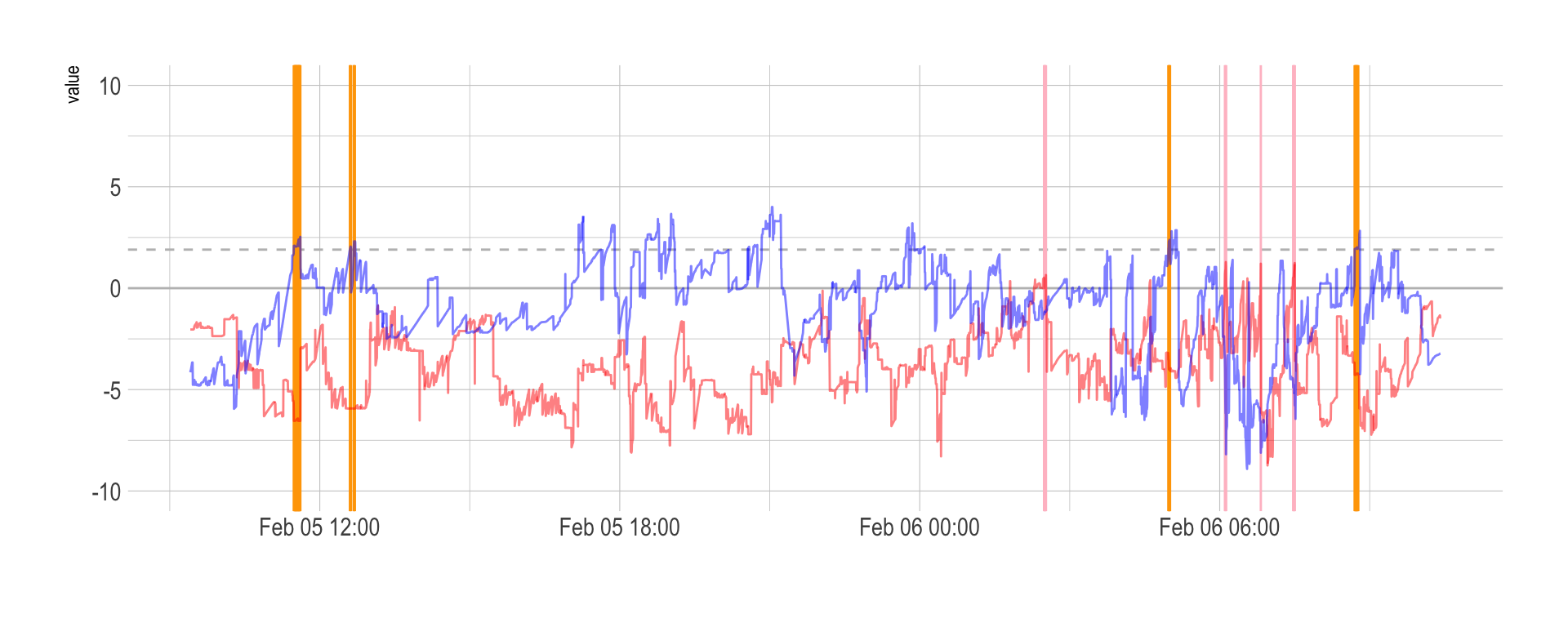

Then we can observe the evolution of the quantity of euro and the quantity of crypto on both platforms. Bitstamp is here represented in red, and Cex is represented in green. At the beginning of the period, Cex is way more expensive than Bitstamp. Thus, several transactions buy bitcoin cash at bitstamp, and sell at Cex. Thus, the amount of euro decreases and quantity of crypto increases for Bitstamp. Exactly the opposite pattern happens for Cex.

# Quantity of euro on both exchanges:
c=bilan %>%
  select(time, euro_plat1, euro_plat2) %>%
  mutate(total=euro_plat1 + euro_plat2) %>%
  gather(plateform, value, -1) %>%
  ggplot( aes(x=time, y=value, color=plateform)) +
    geom_line() +
    theme_ipsum() +
    theme(
      legend.position="none",
      axis.text.x = element_blank(),
      axis.ticks.x = element_blank()
    ) +
    ylab("Quantity of Euro") +
    expand_limits(y=0) +
    xlab("") 
    

# Quantity of crypto on both exchanges
d=bilan %>%
  select(time, crypto_plat1, crypto_plat2) %>%
  mutate(total=crypto_plat1 + crypto_plat2) %>%
  gather(plateform, value, -1) %>%
  ggplot( aes(x=time, y=value, color=plateform)) +
    geom_line() +
    theme_ipsum() +
    theme(
      legend.position="none"
    ) +
    ylab("Quantity of Crypto") +
    expand_limits(y=0) +
    xlab("")

library(patchwork)
c + d + plot_layout(ncol = 1)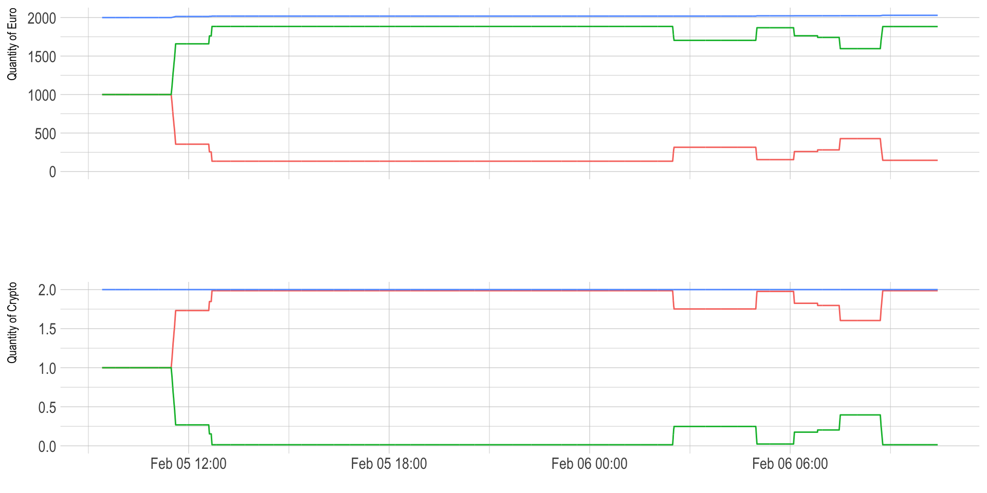

Finally, let’s have a look to the total quantity of euro we got along this process. We started with x euros and end with x euros. This is a benefit of x euros, which is x% of the initial investment. Since this happend on a period of x days, it represent a potential benefit of x% per day.

# Zoom on the total quantity of euro I have
bilan %>%
  ggplot(aes(x=time, y=total_euro)) +
    geom_line(color="black") +
    theme_ipsum() +
    ylab("Total amount of Euro") +
    xlab("")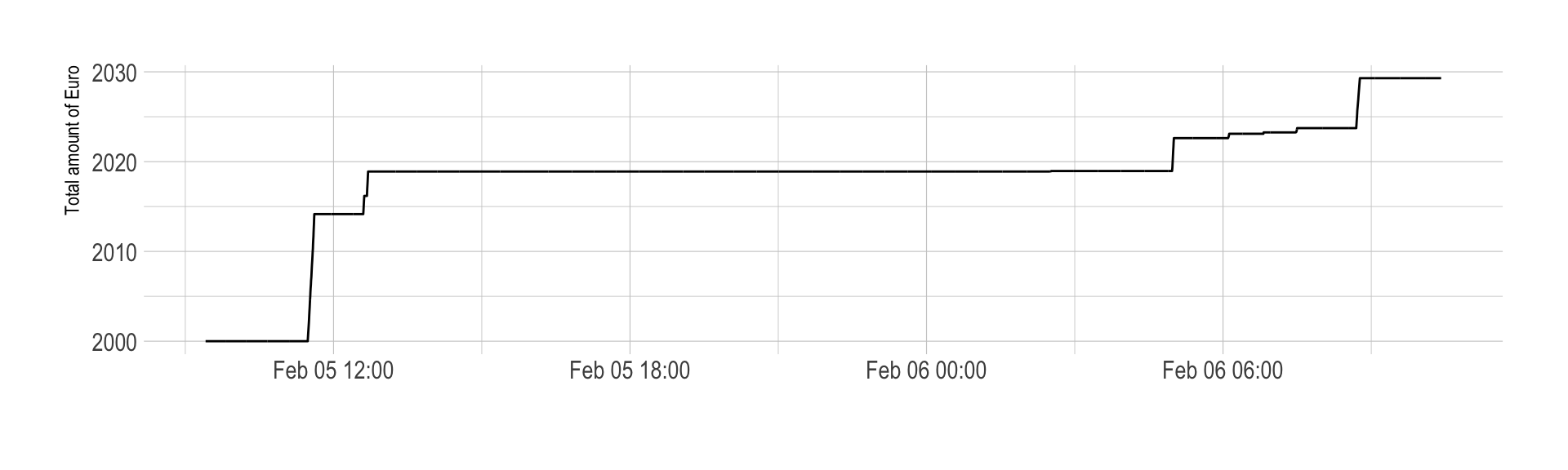

Summary:

# Number of transaction
nb_transac = bilan %>% filter(transaction=="yes") %>% nrow()

# Final amount of money I have
final=bilan$total[nrow(bilan)]

# What I would have without arbitrage
final_without = bilan$total_without_arbitrage[nrow(bilan)]

# Gain compare to no arbitrage in euro, and in % of investment
# --> This is what I have to optimize
diff=final-final_without

# Gain per 24hours?
length = bilan$time[nrow(bilan)] - bilan$time[1]    # In character
length = as.numeric(as.duration(length)) / 3600     # In hours
diff_per_day=24*diff/ length

Optimize the algorithm

The graphics above describe the bot potential behaviour using parameters set up randomly. It traded 20 euros each time the price difference reached a threshold of 1.9%, and rebalanced money whit a threshold of 0.5%.

Let’s run the algorithm using different threshold, to study the impact on the potential profit. The simulation is going to run the bot for a threshold ranging between 0.5 and 3 by 0.2 step, and a rebalancing threshold ranging from -1 to 1 using the same step.

The heatmap below describe the benefit made (in % of the initial investment) according to the thresholds used.

to_try_low= seq(-1,1,0.2)
to_try_high= seq(0.5,3,0.2)
mylen=length(to_try_high)*length(to_try_low)
bilan_optimiz=data.frame(matrix(0,mylen,6))
colnames(bilan_optimiz)=c("lowt", "hight", "nb_transaction", "initial", "final", "diff_perc")
num=0
for(lowt in to_try_low){
  for(hight in to_try_high){
    num=num+1
    #print(paste(lowt, " / ", hight, sep=""))
    result = run_arbitrage_algo(data=data, thres=hight, thres_rebalance=lowt, euro_to_trade=20, initial_value=1000, fee=0.25)
    nb_transaction=result %>% filter(transaction=="yes") %>% nrow()
    final=result$total_euro[nrow(result)]
    initial=1000*2
    diff=final-initial
    diff_perc=diff/initial*100
    
    # write the result
    bilan_optimiz[num,]=c(lowt, hight, nb_transaction, initial, final, diff_perc)    
  }
}

# Plot the result
p <- bilan_optimiz %>%
  mutate(mytext=paste0("Threshold: ", hight, "%\nRebalance: ", lowt, "%\nProfit: ", round(diff_perc,2), "%")) %>%
  ggplot( aes(x=lowt, y=hight, fill=diff_perc, text=mytext) ) +
    geom_tile() + 
    scale_fill_viridis() +
    theme_ipsum() +
    theme(legend.position = "none") +
    xlab("Threshold for rebalancing") +
    ylab("Threshold for arbitrage")
ggplotly(p, tooltip = "text")

One could expect that the best combination of parameters would be the one implying the highest number of transaction. It appears that it is not the case, with an optimal number of transaction to do.

ggplot(bilan_optimiz, aes(x=nb_transaction, y=diff_perc)) +
  geom_point() +
  theme_ipsum() +
  geom_smooth(color="#69b3a2", alpha=0.3) +
  xlab("Number of transaction done") +
  ylab("Benefit realized (in % of investment)")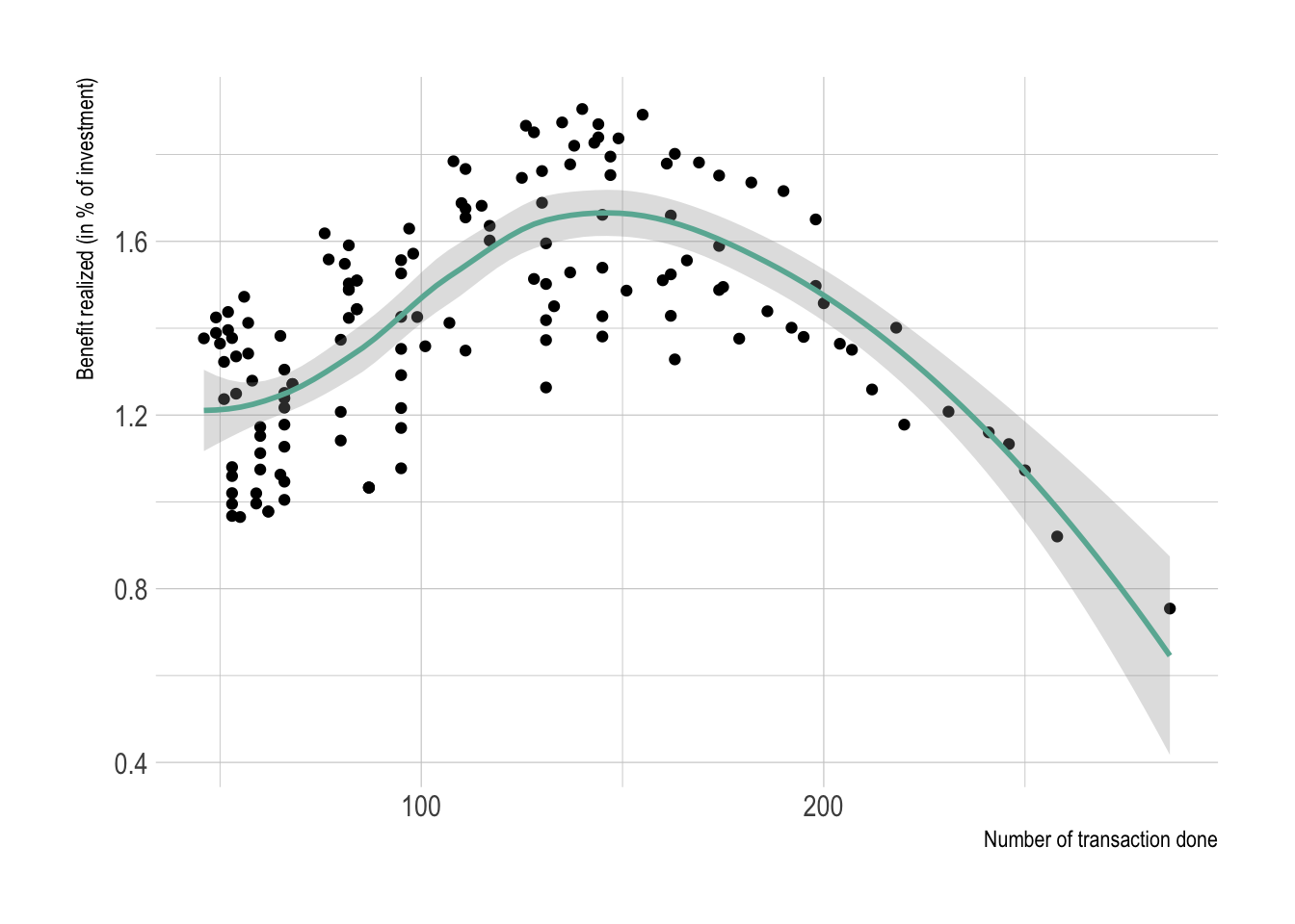

Next step

The next step is to understand what arbitrage is in depth, and study its potential limitations.

< What is arbitrage Calling the private API >