GSMR: testing the putative causal effect of Vitamin-D on about 70 traits
Yan Holtz, Zhihong Zhu, Julanne Frater, Perry Bartlett, Jian Yang, John McGrath
Introduction
GSMR is a tool that allows to run mendelian randomization on summary statistics of GWASs. Basically, its use will test if vitamin-D has a causal effect on other traits and diseases.
The GSMR pipeline requires two types of input file:
Risk factor GWAS - This is the GWAS computed on Vitamin-D concentration and described in the previous tab. Note that waiting for the UKB data, the data of Xia et al. will be used. (sample size of about 80k people).
- Outcome GWASes - GWAS summary statistics for traits potentially influenced by vitamin D concentration. Note that all outcome gwases are listed in supplementary file with their associated publication and main features. 75 traits are considered and divided in three categories.
- Primary traits: 28 traits and diseases with a strong prior for vitamin D effect.
- Secondary traits: 35 traits and diseases with no prior for vitamin D effect.
- Risk factors: 12 traits potentially involved in the mechanism.
Note: cleaning the GWAS summary statistics has been a big work. This step is explained in the script cleaning_GWAS_sumstat.sh
Run GSMR
Step 1: get the last GCTA version that support GSMR. This program is now available on my delta folder at ~/bin/gcta64
Step 2: prepare files - split to have on file per outcome - run GSMR - concatenate results together - transfer result locally. This is done on delta.
# Specific repo
cd /shares/compbio/Group-Wray/YanHoltz/VITAMIND_XIA_ET_AL/3_GSMR

# Prepare a file that gives the location of every b-file (one per chromosome)
ls /gpfs/gpfs01/polaris/Q0286/UKBiobank/v2EURu_HM3/ukbEURu_imp_chr*_v2_HM3_QC.bed | sed 's/.bed//' > gsmr_ref_data.txt

# prepare a file that gives the link to the GWAS result for the risk factor = Vitamin D
echo "vitaminD /shares/compbio/Group-Wray/YanHoltz/DATA/GWAS/XiaEtAl_VitaminD/GWAS_vitaminD_XiaEtAL.ma" > gsmr_exposure.txt

# prepare ONE file that lists all the outcomes. This file has been build in Excel format locally
cd /Users/y.holtz/Dropbox/QBI/4_UK_BIOBANK_GWAS_PROJECT/VitaminD-Causality/0_DATA
R
library(gdata)
tmp <- read.xls("list_of_traits_GSMR.xlsx", header=T)
tmp <- tmp[ , c("Trait","File")]
tmp$File <- paste("/shares/compbio/Group-Wray/YanHoltz/DATA/GWAS/GWAS_SUMSTAT/", tmp$File, sep="")
write.table(tmp, file="list_of_traits_GSMR.txt", row.names=FALSE, quote=FALSE, sep="\t")
q("no")
scp list_of_traits_GSMR.txt y.holtz@delta.imb.uq.edu.au:/shares/compbio/Group-Wray/YanHoltz/VITAMIND_XIA_ET_AL/3_GSMR
cat list_of_traits_GSMR.txt | sed 's/ /_/g' > gsmr_outcome.txt

# Split this file: one file per outcome:
split -l 1 --numeric-suffixes gsmr_outcome.txt
for i in x0* ; do a=$(echo $i | sed 's/x0/x/') ; mv $i $a ; done

# send an array of GSMR
tmp_command="gcta64 --mbfile gsmr_ref_data.txt --gsmr-file gsmr_exposure.txt x{TASK_ID}  --gsmr-direction 0 --out gsmr_result_vitaminDXiaEtAl_{TASK_ID}"
qsubshcom "$tmp_command" 1 30G GSMR_array 10:00:00 "-array=1-72"

# Once it's over, concatenate the results in a unique file
cat gsmr_result_vitaminDXiaEtAl_*gsmr | head -1 > gsmr_result_vitaminDXiaEtAl.gsmr
cat gsmr_result_vitaminDXiaEtAl_*gsmr | grep -v "Exposure" >>  gsmr_result_vitaminDXiaEtAl.gsmr
rm *[0-9].gsmr x* *badsnps qsub* *log

# Then from locally to delta
cd /Users/y.holtz/Dropbox/QBI/4_UK_BIOBANK_GWAS_PROJECT/VitaminD-Causality/0_DATA
scp y.holtz@delta.imb.uq.edu.au:/shares/compbio/Group-Wray/YanHoltz/VITAMIND_XIA_ET_AL/3_GSMR/gsmr_result_vitaminDXiaEtAl.gsmr .
Step 3: read results. Description:
- The exposure is always the Vitamin-D, and we test its causality on several outcomes.
- Bxy is the effect of the exposure on the disease. If this effect is positive, an increase of the exposure creates a increase in the Outcome.
- se is the standard error around Bxy
- p is the pvalue of the association test. We will consider a first threshold of 0.05 for significance, and a second for multiple testing correction (0.05 / # of tests)
- nsnp is the number of SNP with a significant effect on vitamin-D. It is not always the same because a few SNP are sometime discarded by the Heidi outlier test.
# Libraries
library(tidyverse)
library(DT)

# Read gsmr result
gsmr <- read.table("0_DATA/gsmr_result_vitaminDXiaEtAl.gsmr", header = T) %>%
  mutate(Outcome=gsub("_", " ", Outcome))

# Read the meaning of files:
library(gdata)
meaning <- read.xls("0_DATA/list_of_traits_GSMR.xlsx", header=T)
primary <- gsmr %>% filter( Outcome %in% meaning$Trait[ which(meaning$Group=="Primary") ] )
secondary <- gsmr %>% filter( Outcome %in% meaning$Trait[ which(meaning$Group=="Secondary") ] )
risk <- gsmr %>% filter( Outcome %in% meaning$Trait[ which(meaning$Group=="Risk") ] )

# Compute thresholds
thres_primary <- 0.05 / nrow(primary)
thres_secondary <- 0.05 / nrow(secondary)
thres_risk <- 0.05 / nrow(risk)
Result: primary traits
In total 27 primary traits were studied. The threshold used to take multiple testing into account is 0.05 / # of test. Here is a description of the effect size and pvalues obtained with the GSMR test:
Effect size
The following chart describes the effect sizes (bxy) of vitamin D on each primary traits. The standard error is indicated in green.
#plot
primary %>%
  arrange(bxy) %>%
  filter(!is.na(bxy) ) %>%
  mutate(name=factor(Outcome, unique(Outcome))) %>%
  mutate(significance=ifelse(p<thres_primary, "signif multi.testing", ifelse(p<0.05, "signif", "nonSignif") ) ) %>%
  ggplot( aes(x=name, y=bxy)) +
    geom_hline( yintercept=0 ) +
    geom_segment( aes(x=name, xend=name, y=bxy-se, yend=bxy+se), color="grey", alpha=0.7) +
    geom_point(aes(color=significance), size=4) +
    scale_color_manual( values=c("grey", "orange", "red")) +
    coord_flip() +
    theme_bw() +
    theme( panel.grid.major.y = element_line(size=0.1)) +
    ylab("Bxy (Effect size)") +
    xlab("")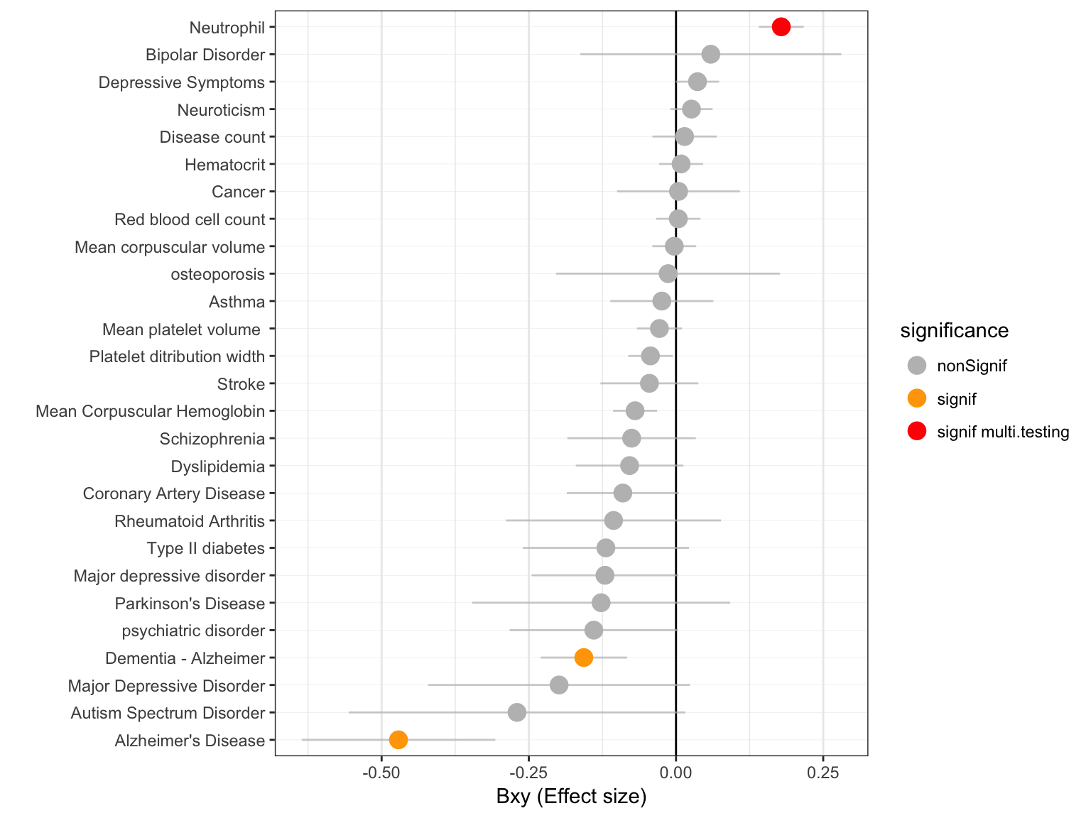
Figure: effect size (Bxy) of Vitamin D on all primary traits. Grey / orange / red points show significance of the causality. Blue lines show the standard error around the effect size.
#Save at png
ggsave(filename = "IMG/gsmrPrimaryTraits.png")
A few observation:
- most of the effect size are negative: in these cases a lack of vitamin D increase the chances to develop a disease.
- few effect are significant. This is probably due to the fact that the number of genetic instrument is currently very low (6 significant SNPs only)
- it is interesting to note the strong association between vitamin D and
Alzheimer's disease. Two GWAS are available for this disease and both give a significant result.
Pvalues
Here is an ordered barplot of the pvalues. We have several traits over the 0.05 threshold of significance. But this does not account for multiple testing.
primary %>%
  arrange(desc(p)) %>%
  filter( !is.na(bxy)) %>%
  mutate(name=factor(Outcome, unique(Outcome))) %>%
  mutate(significance=ifelse(p<thres_primary, "signif multi.testing", ifelse(p<0.05, "signif", "nonSignif") ) ) %>%
  ggplot( aes(x=name, y=-log10(p))) +
    geom_segment( aes(x=name, xend=name, y=-log10(p), yend=0), color="grey", alpha=0.7) +
    geom_point(aes(color=significance), size=4) +
    scale_color_manual( values=c("grey", "orange", "red")) +
    coord_flip() +
    theme_light() +
    theme( panel.grid.major.y = element_blank()) +
    ylab("-log10( pvalue )") +
xlab("") 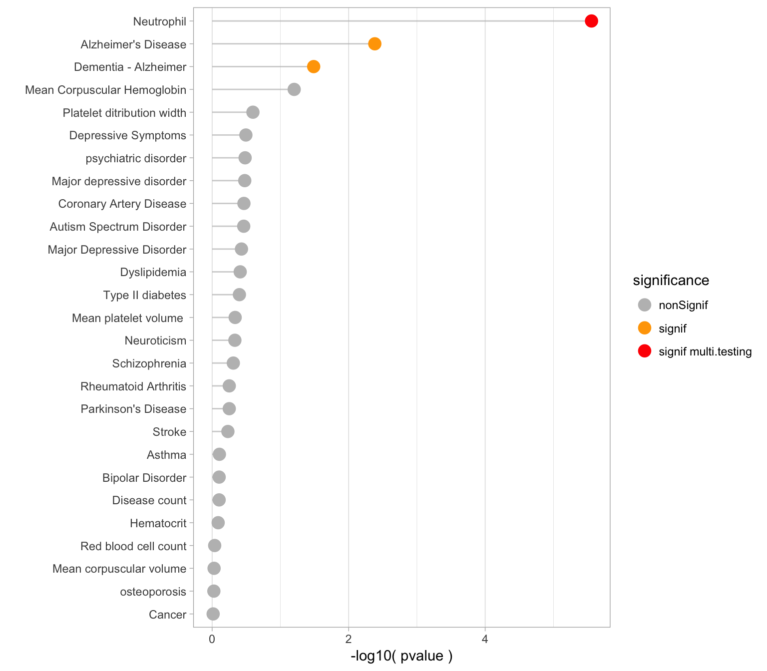
Result: secondary traits
In total 27 primary traits were studied. The threshold used to take multiple testing into account is 0.05 / # of test. Here is a description of the effect size and pvalues obtained with the GSMR test:
Effect size
# Plot
secondary %>%
  arrange(bxy) %>%
  filter(!is.na(bxy) ) %>%
  mutate(name=factor(Outcome, unique(Outcome))) %>%
  mutate(significance=ifelse(p<thres_secondary, "signif multi.testing", ifelse(p<0.05, "signif", "nonSignif") ) ) %>%
  ggplot( aes(x=name, y=bxy)) +
    geom_hline( yintercept=0 ) +
    geom_segment( aes(x=name, xend=name, y=bxy-se, yend=bxy+se), color="grey", alpha=0.7) +
    geom_point(aes(color=significance), size=4) +
    scale_color_manual( values=c("grey", "orange", "red")) +
    coord_flip() +
    theme_bw() +
    theme( panel.grid.major.y = element_line(size=0.1)) +
    ylab("Bxy (Effect size)") +
    xlab("")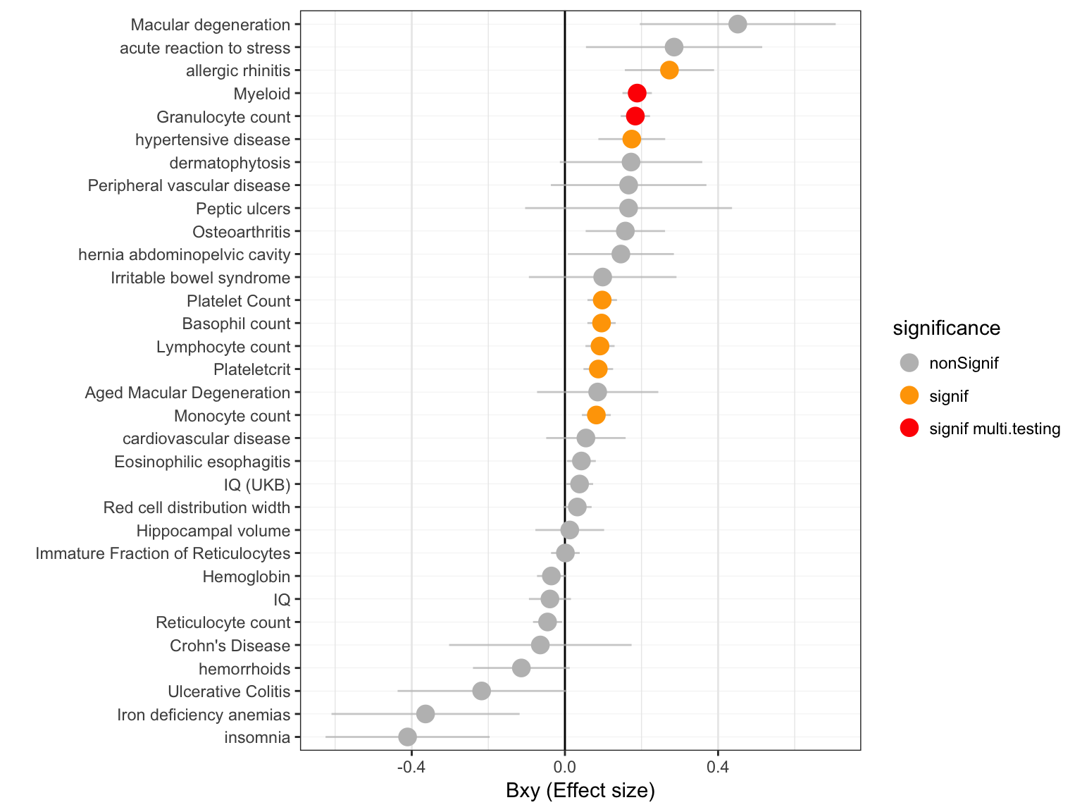
Figure: effect size (Bxy) of Vitamin D on all primary traits. Grey / orange / red points show significance of the causality. Blue lines show the standard error around the effect size.
#Save at png
ggsave(filename = "IMG/gsmrSecondaryTraits.png")
A few observation:
- 2 significant associations after multiple testing correction.
- 2 of have a positive effect size: more Vitamin-D, more trait.
- 0 have a negative effect size.
Pvalues
Here is an ordered barplot of the pvalues. We have several traits over the 0.05 threshold of significance. But this does not account for multiple testing.
secondary %>%
  arrange(desc(p)) %>%
  filter( !is.na(bxy)) %>%
  mutate(name=factor(Outcome, unique(Outcome))) %>%
  mutate(significance=ifelse(p<thres_secondary, "signif multi.testing", ifelse(p<0.05, "signif", "nonSignif") ) ) %>%
  ggplot( aes(x=name, y=-log10(p))) +
    geom_segment( aes(x=name, xend=name, y=-log10(p), yend=0), color="grey", alpha=0.7) +
    geom_point(aes(color=significance), size=4) +
    scale_color_manual( values=c("grey", "orange", "red")) +
    coord_flip() +
    theme_light() +
    theme( panel.grid.major.y = element_blank()) +
    ylab("-log10( pvalue )") +
xlab("") 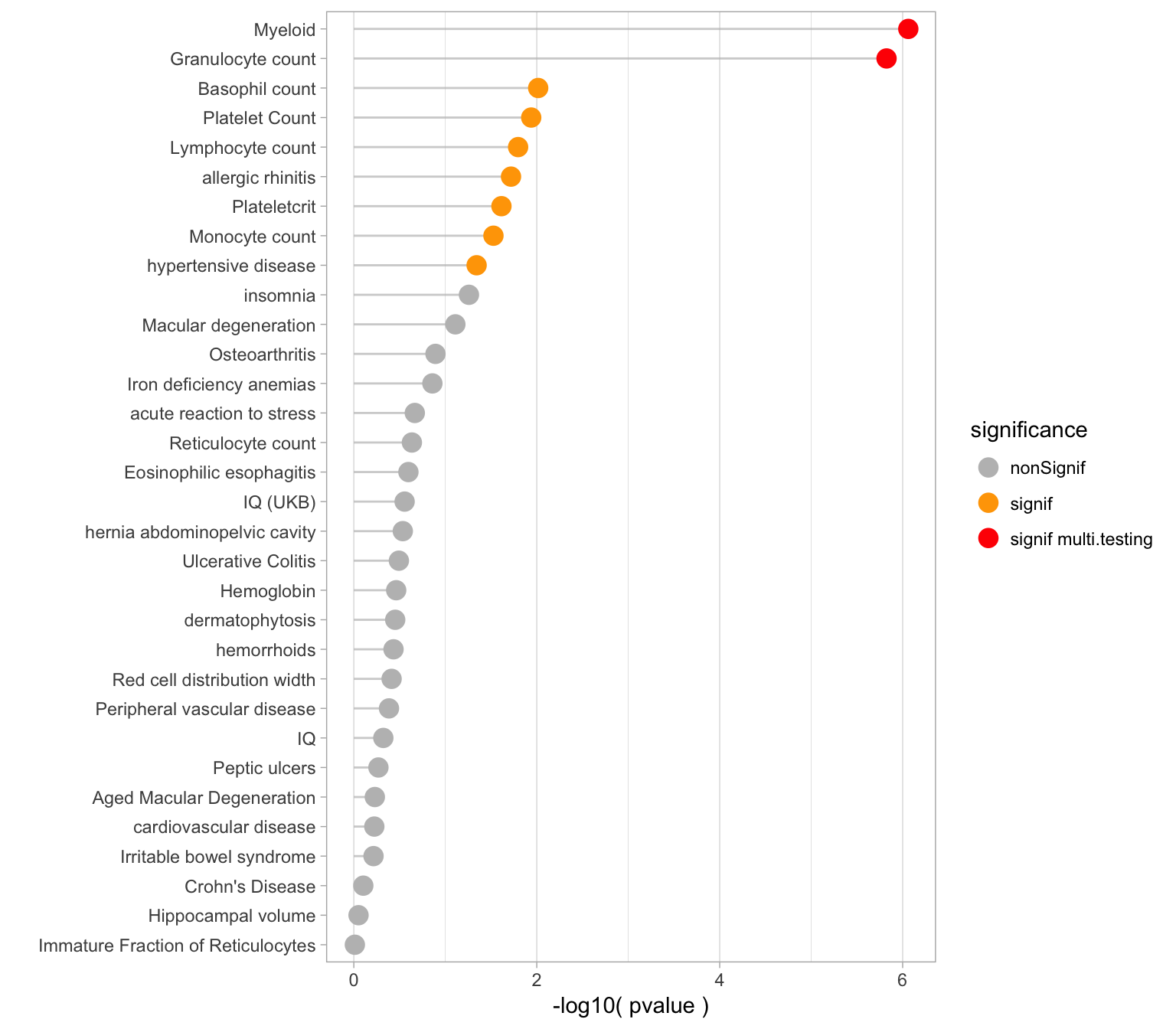
Result: Risk factors
Effect size
A few observation:
- 1 significant associations after multiple testing correction.
- 1 of have a positive effect size: more Vitamin-D, more trait.
- 0 have a negative effect size.
#plot
risk %>%
  arrange(bxy) %>%
  filter(!is.na(bxy) ) %>%
  mutate(name=factor(Outcome, unique(Outcome))) %>%
  mutate(significance=ifelse(p<thres_risk, "signif multi.testing", ifelse(p<0.05, "signif", "nonSignif") ) ) %>%
  ggplot( aes(x=name, y=bxy)) +
    geom_hline( yintercept=0 ) +
    geom_segment( aes(x=name, xend=name, y=bxy-se, yend=bxy+se), color="skyblue", alpha=0.7) +
    geom_point(aes(color=significance), size=4) +
    scale_color_manual( values=c("grey", "orange", "red")) +
    coord_flip() +
    theme_bw() +
    theme( panel.grid.major.y = element_line(size=0.1)) +
    ylab("Bxy (Effect size)") +
    xlab("")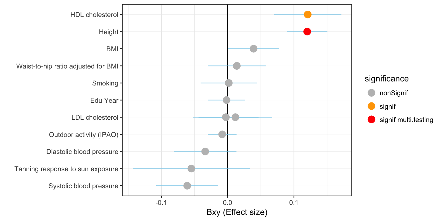
Figure: effect size (Bxy) of Vitamin D on all primary traits. Grey / orange / red points show significance of the causality. Blue lines show the standard error around the effect size.
#Save at png
ggsave(filename = "IMG/gsmrRiskFactors.png")
Pvalues
Here is an ordered barplot of the pvalues. We have several traits over the 0.05 threshold of significance. But this does not account for multiple testing.
risk %>%
  arrange(desc(p)) %>%
  filter( !is.na(bxy)) %>%
  mutate(name=factor(Outcome, unique(Outcome))) %>%
  mutate(significance=ifelse(p<thres_risk, "signif multi.testing", ifelse(p<0.05, "signif", "nonSignif") ) ) %>%
  ggplot( aes(x=name, y=-log10(p))) +
    geom_segment( aes(x=name, xend=name, y=-log10(p), yend=0), color="skyblue", alpha=0.7) +
    geom_point(aes(color=significance), size=4) +
    scale_color_manual( values=c("grey", "orange", "red")) +
    coord_flip() +
    theme_light() +
    theme( panel.grid.major.y = element_blank()) +
    ylab("-log10( pvalue )") +
xlab("") 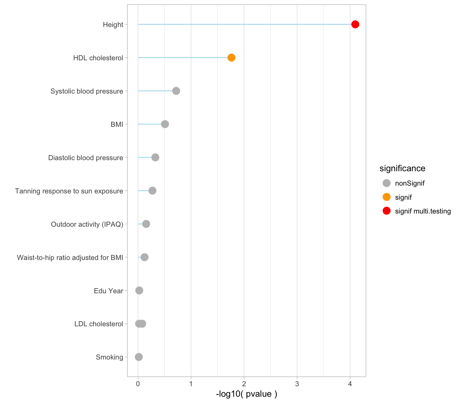
Table
The 71 GSMR test results are displayed in this table in case you need to check a specific value:
datatable(gsmr %>% arrange(p), rownames = FALSE, options = list(pageLength = 10) )Reverse GSMR
Work in progress
# Specific repo
cd /shares/compbio/Group-Wray/YanHoltz/VITAMIND_XIA_ET_AL/3_GSMR/REVERSE

# Prepare a file that gives the location of every b-file (one per chromosome) --> I don't take hapmap3, cauz may be the signif SNP are not in Hapmap3
ls /gpfs/gpfs01/polaris/Q0286/UKBiobank/v2EUR_geno/ukbEUR_cal_chr*_v2_QC.bed | sed 's/.bed//' > gsmr_ref_data.txt

# copy GWAS sumstat files done for the forward GSMR
cp ../gsmr_exposure.txt ../gsmr_outcome.txt .

# Split this file: one file per outcome:
split -l 1 --numeric-suffixes gsmr_outcome.txt
for i in x0* ; do a=$(echo $i | sed 's/x0/x/') ; mv $i $a ; done

# send an array of GSMR
tmp_command="gcta64 --mbfile gsmr_ref_data.txt --gsmr-file gsmr_exposure.txt x{TASK_ID}  --gsmr-direction 1 --out gsmr_reverse_result_vitaminDXiaEtAl_{TASK_ID}"
qsubshcom "$tmp_command" 1 30G GSMR_array 10:00:00 "-array=1-72"

# Once it's over, concatenate the results in a unique file
cat gsmr_reverse_result*gsmr | head -1 > gsmr_reverse_result_vitaminDXiaEtAl.gsmr
cat gsmr_reverse_result*gsmr | grep -v "Exposure" >>  gsmr_reverse_result_vitaminDXiaEtAl.gsmr
rm *[0-9].gsmr x* *badsnps qsub*
- Conclusion
- GSMR analysis suggests that vitamin-D concentration has a causal effect on several traits like Hypertension or Alzheimer. This sould be verified using a bigger sample size and multiple testing correction.
A work by Yan Holtz
Yan.holtz.data@gmail.com