Run the GWAS
Data
Running a GWAS requires several information:
a phenotype file: the phenotype file created by the script in the previous page: /home/y.holtz/BLOOD_GWAS/0_DATA/pheno.txt.gz. It has one line per individual. Its first column is the individual id. Other columns are traits. Traits include the Diastolic blood pressure, field 4079 of the UKB.
- a genotype file: gives the alleles at each variants for each individual. Several version exist. HapMap3 has about 2M SNPs. I used the file
/afm01/Q0286/UKBiobank/v2EURu_HM3, it keeps only unrelated European people. Note that information is stored using a compressed format and is thus split in three files:
- .bed (alleles coded 0, 1, 2),
- .fam (detail of each SNP like id, cM, bP, All1 and All2),
- .bin (detail of each individual (id mainly).
a list of PCs: used to correct for the population structure in plink only. Several PCs are available: computed on 1000 genomes, computed on the UKB… In my analysis I used:
Plink
I run plink version 1.9 for this analysis. Option used are:
- allow-no-sex: explanation:
- linear
- PCs correction
An array is used to send the calculation for each chromosome in parrallele. This is done thanks to this script.
# Good folder on delta
cd /shares/compbio/Group-Wray/YanHoltz/IPAQ_GWAS

# prepare command
tmp_command="plink \
          --bfile /gpfs/gpfs01/polaris/Q0286/UKBiobank/v2EURu_HM3/ukbEURu_imp_chr{TASK_ID}_v2_HM3_QC\
          --allow-no-sex \
          --linear \
          --pheno /shares/compbio/Group-Wray/YanHoltz/DATA/PHENOTYPE/UKB/UKB_IPAQ_score.txt \
          --pheno-name IPAQ \
          --out GWAS_IPAQ_{TASK_ID}"

# Send command in qsub
qsubshcom "$tmp_command" 1 30G GWAS_plink 10:00:00 "-array=1-22"
I need to make 3 files at the end of this GWAS:
- A first output file for clumping and general description. It is just a concatenation of all the individual chromosome outputs.
# Make the file
cd /home/y.holtz/BLOOD_GWAS/1_GWAS/PLINK
head -1 GWAS_blood_pressure_1.assoc.linear  > tmp
cat GWAS*linear | grep -v 'CHR'   >> tmp

# Remove weird spaces
cat tmp | awk '{ print $1,$2,$3,$4,$5,$6,$7,$8,$9 }' > result_GWAS_bloodpressure_plink.linear
gzip result_GWAS_bloodpressure_plink.linear
- A .ma file that will be used by SMR and GSMR
# first I need to compute the allele frequency of the reference allele with gcta (~30 minutes)
cd /home/y.holtz/BLOOD_GWAS/1_GWAS
tmp_command="gcta64 --bfile /gpfs/gpfs01/polaris/Q0286/UKBiobank/v2EURu_HM3/ukbEURu_imp_chr{TASK_ID}_v2_HM3_QC --freq --out all_frequency_{TASK_ID}"
qsubshcom "$tmp_command" 1 30G allFreq_GCTA 10:00:00 "-array=1-22"

# Now I can build the .ma file for GSMR
echo "SNP A1 A2 freq b se p n" > GWAS_blood_pressure.ma
join <(awk '{print $2, $5, $6}' /gpfs/gpfs01/polaris/Q0286/UKBiobank/v2EURu_HM3/ukbEURu_imp_chr*bim | sort -k 1,1) <(awk '{print $2, $6}' all_frequency*.frq | sort) | join - <(zcat result_GWAS_bloodpressure_plink.linear.gz | awk '{if(NR>1) print $2, $7, $7/$8, $9, $6 }' | sort -k 1,1) >> GWAS_blood_pressure.ma
- A ‘light weight’ version for sharing with others, compute a few analysis, and use online plateforms. I keep only SNPs with a pvalue < 0.05
m
Bolt
Bolt takes into account the population structure: it computes a genomic relationship matrix (GMR) from the genotype file and use it in the GWAS model. It thus takes way longer than plink, but gives a more precise result. It needs the whole genomic to compute the GMR, thus this analysis cannot be run on one chromosome only.
See code below to run the bolt analysis:
# Go to the appropriate folder:
cd /shares/compbio/Group-Wray/YanHoltz/IPAQ_GWAS/BOLT

# A list of the files I need to run the GWAS:
bolt="/gpfs/gpfs01/polaris/Q0286/bin/ukb_gwas_tool/bin/BOLT-LMM_v2.3/bolt"
phen="/shares/compbio/Group-Wray/YanHoltz/DATA/PHENOTYPE/UKB/UKB_IPAQ_score.txt"
trait="IPAQ"

# SNP to exclude: I discard SNP with MAF <0.001
exsnp="/gpfs/gpfs01/polaris/Q0286/UKBiobank/v2EUR_impHRC/ukbEUR_imp_all_v2_imp_QC_HRC_maf0001.EXCLUDEvarList"

# Genotyping file = whole european HRC SNP = ~28730907 SNPs
bim="/gpfs/gpfs01/polaris/Q0286/UKBiobank/v2EUR_impHRC/ukbEUR_imp_chr{1:22}_v2_imp_QC_HRC.bim"
bed="/gpfs/gpfs01/polaris/Q0286/UKBiobank/v2EUR_impHRC/ukbEUR_imp_chr{1:22}_v2_imp_QC_HRC.bed"
fam="/gpfs/gpfs01/polaris/Q0286/UKBiobank/v2EUR_impHRC/ukbEUR_imp_chr1_v2_imp_QC_HRC.fam"

# Covariate: sex age and 10 PCs. Note, it is also possible to correct for these traits before bolt.
covar="/gpfs/gpfs01/polaris/Q0286/uqaxue/phen/covar_sex_age_10PCs.txt"

# LDScore of each SNP (8M SNPs) -> used to compute the GRM
table="/gpfs/gpfs01/polaris/Q0286/uqaxue/bin/BOLT/tables/LDSCORE.1000G_EUR.tab.gz"

# Relation cM / Mb -> used for the GRM as well
map="/gpfs/gpfs01/polaris/Q0286/uqaxue/bin/BOLT/tables/genetic_map_hg19.txt.gz"

# list of SNP for the GRM = pruned SNP selection from HapMap3
j_hm3="/gpfs/gpfs01/polaris/Q0286/uqaxue/phen/ukbEURu_imp_v2_HM3_QC_R2_09.snplist"

out="/shares/compbio/Group-Wray/YanHoltz/IPAQ_GWAS/BOLT/GWAS_IPAQ_bolt.txt"

# Send the script
tmp_command="$bolt --bed=$bed --bim=$bim --fam=$fam --exclude $exsnp --phenoFile=$phen --phenoCol=$trait --covarFile $covar --covarCol=Sex --qCovarCol=Age --qCovarCol=PC{1:10} --lmm --modelSnps=$j_hm3 --maxModelSnps=720000 --LDscoresFile=$table --geneticMapFile=$map --statsFile=$out --numThreads 16"

# Send command
qsubshcom "$tmp_command" 1 100G GWAS_bolt 60:00:00 ""
I need to make 3 files at the end of this GWAS:
- .linear: A first output file for clumping and general description. It will look like plink output.
# Make the file
cd /home/y.holtz/BLOOD_GWAS/1_GWAS/BOLT
echo "CHR SNP BP A1 TEST NMISS BETA STAT P" > result_GWAS_bloodpressure_bolt.linear
cat output.res | grep -v '^SNP' | awk '{print $2, $1, $3, $5, "ADD", "300000", $9, $9/$10, $11 }'   >> result_GWAS_bloodpressure_bolt.linear
gzip result_GWAS_bloodpressure_bolt.linear
- .ma: file that will be used by SMR and GSMR
# !! to make the .ma file I need the number of available individual per SNP. This is not so easy. Angli has done a script for that.
# See mail sended. See the script in /shares/compbio/Group-Wray/YanHoltz/SOFT/clean_BOLT_output.R
# Just need to reorder column + go from missing data frequency to Number of available individual.
more /shares/compbio/PCTG/a.xue/for_Yan/ukbEUR_MAF1e-4_IPAQG.bolt |  awk '{ print $1, $5, $6, $7, $9, $10, $11, 456426*(1-$8) }' | more
- light weight version for sharing with others, compute a few analysis, and use online plateforms. I keep only SNPs with a pvalue < 0.05
zcat result_GWAS_bloodpressure_bolt.linear.gz | head -1 > result_GWAS_bloodpressure_bolt.linear.light
zcat result_GWAS_bloodpressure_bolt.linear.gz | awk '{ if($9<0.05){print $0 }}' >> result_GWAS_bloodpressure_bolt.linear.light
gzip result_GWAS_bloodpressure_bolt.linear.light
- Split per chromosome: to run the clumping faster, it is more convenient to have 1 file per chromosome.
for i in $(seq 1 22); do
  echo $i ;
  zcat  result_GWAS_bloodpressure_bolt.linear.gz | head -1 > result_GWAS_bloodpressure_bolt_$i.linear
  zcat  result_GWAS_bloodpressure_bolt.linear.gz | grep ^${i} >> result_GWAS_bloodpressure_bolt_$i.linear
done
Transfer files locally:
cd /Users/y.holtz/Dropbox/QBI/4_UK_BIOBANK_GWAS_PROJECT/VitaminD-GWAS/0_DATA
scp  y.holtz@delta.imb.uq.edu.au:/home/y.holtz/BLOOD_GWAS/1_GWAS/BOLT/result_GWAS_bloodpressure_bolt.linear.gz  .
Clumping
Once I have the GWAS result, I have to ‘clump’ it: I find all the independant pics of association, find the highest LOD, the markers involved in this pic, the position of the pic… What does it take into account? It considers:
- LOD score of each SNP
- LD between SNPs
- Physical distance between SNPs.
Here are the clumping options I’ve used:
- p1 is the Significance threshold for an association
- p2 is Secondary significance threshold for clumped SNPs = SNPs that are part of the association, but not pic.
- r2 is the LD threshold for clumping and
- clump-kb is the physical distance threshold for clumping
Plink
# good folder
cd /home/y.holtz/BLOOD_GWAS/2_CLUMPING/PLINK

# Prepare command
tmp_command="plink \
          --bfile /gpfs/gpfs01/polaris/Q0286/UKBiobank/v2EURu_HM3/ukbEURu_imp_chr{TASK_ID}_v2_HM3_QC\
          --clump /home/y.holtz/BLOOD_GWAS/1_GWAS/PLINK/GWAS_blood_pressure_{TASK_ID}.assoc.linear \
          --clump-p1 0.00000001 --clump-r2 0.50 --clump-kb 500 \
          --out /home/y.holtz/BLOOD_GWAS/2_CLUMPING/PLINK/CLUMP_bloodpressure_{TASK_ID}.txt"

# Send qsub
qsubshcom "$tmp_command" 1 30G clumping_plink 10:00:00 "-array=1-22"

#It is more handy to have only one file with all the chromosome. Let's build it:
cat *clumped | grep "CHR" | head -1 > result_GWAS_bloodpressure_plink_clumped
cat CLUMP*clumped | grep -v "CHR" |sed '/^$/d'  >> result_GWAS_bloodpressure_plink_clumped
Bolt
# good folder
cd /home/y.holtz/BLOOD_GWAS/2_CLUMPING/BOLT

# Prepare command
tmp_command="plink \
          --bfile /gpfs/gpfs01/polaris/Q0286/UKBiobank/v2EURu_HM3/ukbEURu_imp_chr{TASK_ID}_v2_HM3_QC\
          --clump /home/y.holtz/BLOOD_GWAS/1_GWAS/BOLT/result_GWAS_bloodpressure_bolt_{TASK_ID}.linear\
          --clump-p1 0.00000001 --clump-r2 0.50 --clump-kb 500 \
          --out /home/y.holtz/BLOOD_GWAS/2_CLUMPING/BOLT/CLUMP_bloodpressure_{TASK_ID}_bolt.txt"

# Send qsub
qsubshcom "$tmp_command" 1 30G clumping_bolt 10:00:00 "-array=1-22"

#It is more handy to have only one file with all the chromosome. Let's build it:
cat *clumped | grep "CHR" | head -1 > result_GWAS_bloodpressure_bolt_clumped
cat CLUMP*clumped | grep -v "CHR" | grep -v "NA" | sed '/^$/d'  >> result_GWAS_bloodpressure_bolt_clumped
# Transfert it locally
cd /Users/y.holtz/Dropbox/QBI/4_UK_BIOBANK_GWAS_PROJECT/VitaminD-GWAS/0_DATA
scp  y.holtz@delta.imb.uq.edu.au:/home/y.holtz/BLOOD_GWAS/2_CLUMPING/BOLT/result_GWAS_bloodpressure_*_clumped  .
Plink GWAS Result
# Read result
data=read_delim("0_DATA/GWAS_vitaminD_XiaEtAL.linear.gz", col_names=T, delim=" ")
data$CHR=as.factor(data$CHR)
#data=data %>% sample_n(500000)

# Read after clumping data
clump=read.table("0_DATA/result_GWAS_VitaminD_XiaEtAl_clumped", header=T)

# A list of all SNPs implicated in an association?
Hit_SNP <- c(
  as.character(clump$SNP),
  strsplit(as.character(clump$SP2), ',', fixed=TRUE) %>% unlist() %>% gsub("\\(.\\)", "", .)
)
Hit_SNP <- Hit_SNP[Hit_SNP != "NONE"]
Manhattan
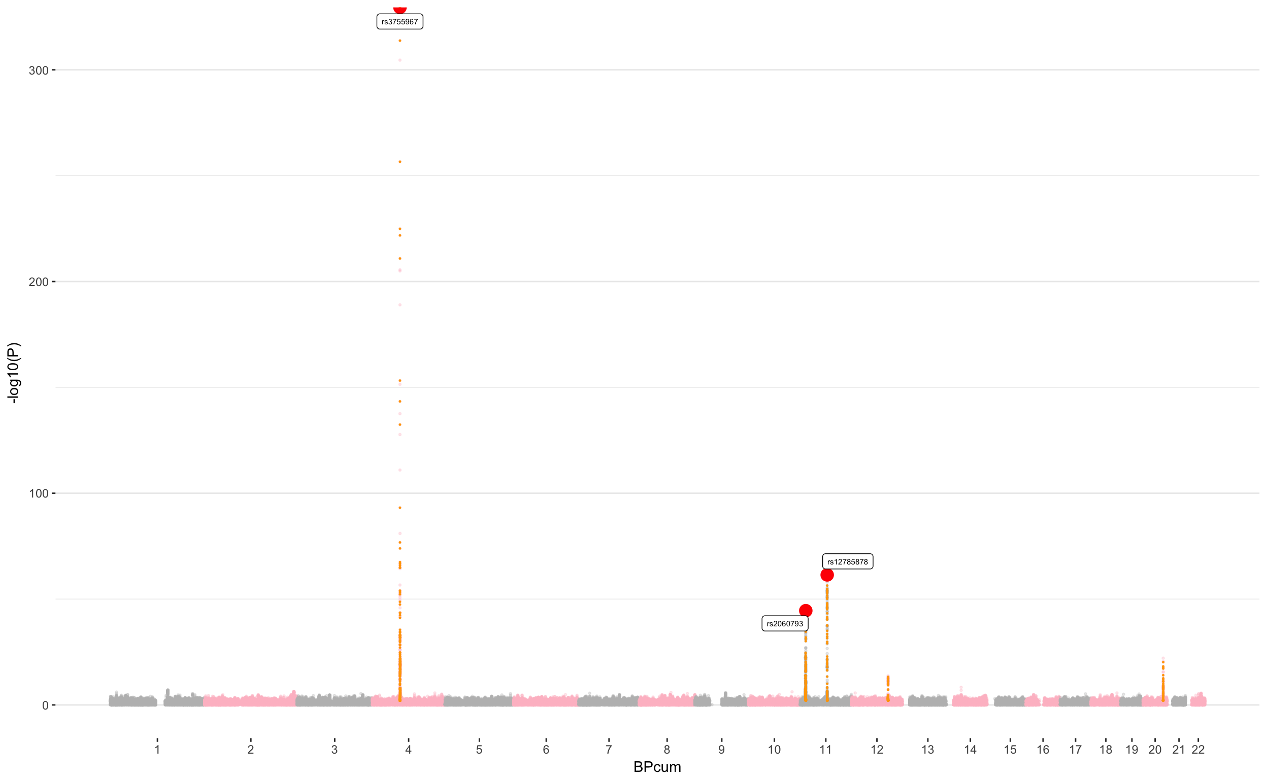
Most common Manhattan plot
# -------- Add cumulative position + clumping information to data
don <- data %>%

  # Compute chromosome size and merge this info to the GWAS result
  group_by(CHR) %>%
  summarise(chr_len=max(BP)) %>%
  mutate(tot=cumsum(chr_len)-chr_len) %>%
  dplyr::select(-chr_len) %>%
  left_join(data, ., by=c("CHR"="CHR")) %>%

  # keep only SNP with pvalue < 0.05: it makes the plot realisation way faster
  filter( P<0.03 | SNP %in% sample(data$SNP, 100000)) %>%

  # Add a cumulative position colummn to the data set
  arrange(CHR, BP) %>%
  mutate( BPcum=BP+tot) %>%

  # Add clumping information
  mutate( is_major=ifelse(SNP %in% clump$SNP & P<0.0000000000000000000001, "yes", "no")) %>%
  mutate( is_clump=ifelse(SNP %in% Hit_SNP, "yes", "no"))


# -------- prepare X axis
axisdf = don %>% group_by(CHR) %>% summarize(center=( max(BPcum) + min(BPcum) ) / 2 )


# -------- Make the plot
ggplot(don, aes(x=BPcum, y=-log10(P))) +

    # Show all points
    geom_point( aes(color=as.factor(CHR)), alpha=0.3, size=0.5) +
    scale_color_manual(values = rep(c("grey", "pink"),44)) +

    # Add highlighted points for significant association:
    geom_point(data=subset(don, is_clump=="yes"), color="orange", size=0.2) +
    geom_point(data=subset(don, is_major=="yes"), color="red", size=4) +
    geom_label_repel( data=subset(don, is_major=="yes"), aes(label=SNP), size=2) +

    # Make X axis:
    scale_x_continuous( label = axisdf$CHR, breaks= axisdf$center ) +

    theme_bw() +
    theme(
      legend.position="none",
      panel.border = element_blank(),
      panel.grid.major.x = element_blank(),
      panel.grid.minor.x = element_blank()
    )

Main statistics
nb_snp=nrow(data)
signif = data %>% filter(P<0.00000001) %>% arrange(CHR, BP)
nb_signif=nrow(signif)
We had 2543566 in our data set. We found 522 significant association (with a 10^-8 threshold).
Here is a list of all the significant assoc:
datatable(signif, rownames = FALSE, options = list(pageLength = 5) )
Clumping details
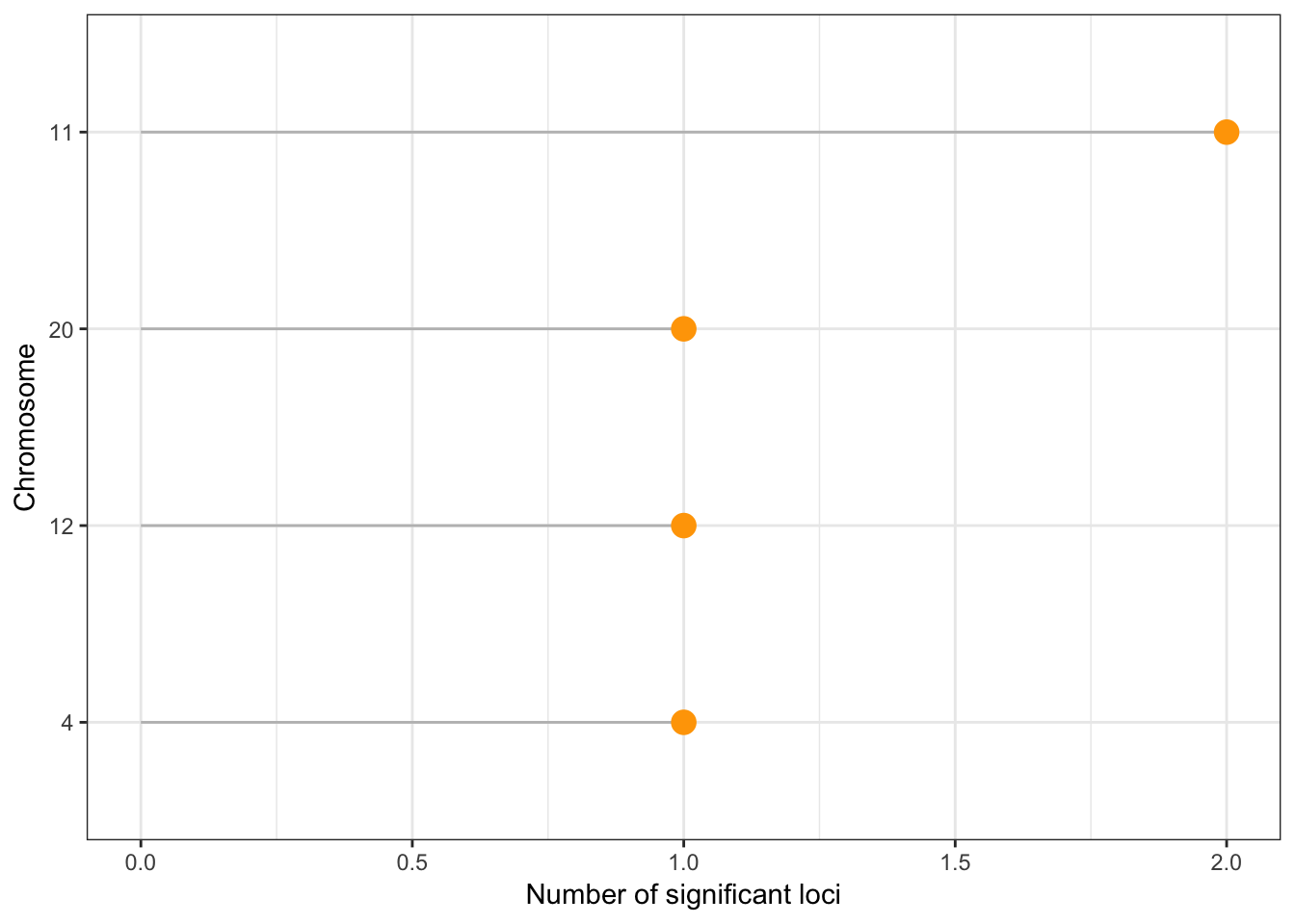
Number of unique significant loci detected after clumping: 5 Number of loci per chromosome:
clump %>%
  group_by(CHR) %>%
  summarise( tot=n() ) %>%
  arrange(tot) %>%
  mutate(CHR=factor(CHR, CHR)) %>%
  ggplot( aes(x=CHR, y=tot)) +
    geom_segment(aes(x=CHR, xend=CHR, y=tot, yend=0), color="grey") +
    geom_point(size=4, color="orange") +
    coord_flip() +
    ylab("Number of significant loci") +
    xlab("Chromosome") +
    theme_bw()

Detail of the clumping results:
datatable(clump, rownames = FALSE, options = list(pageLength = 5) )
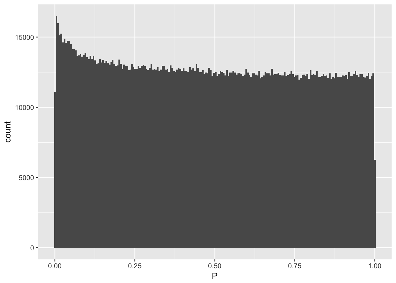
Pvalue distribution
data %>% ggplot(aes(x=P)) + geom_histogram(bins=200)

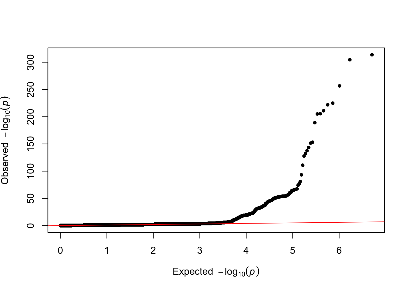
QQplot
qq(data$P)

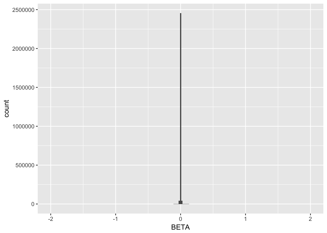
Beta distribution
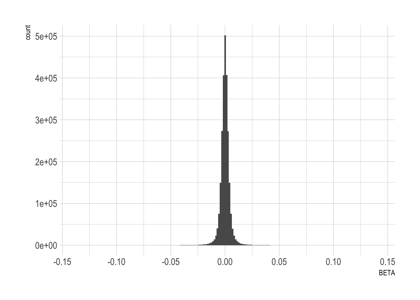
Should be a normal distribution centered on 0? If Beta=0, the SNP has no effect. If absolute(Beta) is strong, SNP has a strong effect.
data %>% ggplot(aes(x=BETA)) + geom_histogram(bins=200) + theme_ipsum() #+ xlim(-2,2)

Bolt GWAS Result
# Read result
#data=read_delim("0_DATA/GWAS_vitaminD_XiaEtAL.linear.gz", col_names=T, delim=" ")
#data$CHR=as.factor(data$CHR)
#data=data[ sample(seq(1,nrow(data)), 10000) , ]

# Read after clumping data
clump=read.table("0_DATA/result_GWAS_VitaminD_XiaEtAl_clumped", header=T)
clump <- clump %>% filter(P<10e-8)

# A list of all SNPs implicated in an association?
Hit_SNP <- c(
  as.character(clump$SNP),
  strsplit(as.character(clump$SP2), ',', fixed=TRUE) %>% unlist() %>% gsub("\\(.\\)", "", .)
)
Hit_SNP <- Hit_SNP[Hit_SNP != "NONE"]
Manhattan
Most common Manhattan plot
# -------- Add cumulative position + clumping information to data
don <- data %>%

  # Compute chromosome size and merge this info to the GWAS result
  group_by(CHR) %>%
  summarise(chr_len=max(BP)) %>%
  mutate(tot=cumsum(chr_len)-chr_len) %>%
  dplyr::select(-chr_len) %>%
  left_join(data, ., by=c("CHR"="CHR")) %>%

  # keep only SNP with pvalue < 0.05: it makes the plot realisation way faster
  #filter( P<0.05 | SNP %in% sample(data$SNP, 70000)) %>%

  # Add a cumulative position colummn to the data set
  arrange(CHR, BP) %>%
  mutate( BPcum=BP+tot) %>%

  # Add clumping information
  mutate( is_major=ifelse(SNP %in% clump$SNP & P<10e-15, "yes", "no")) %>%
  mutate( is_clump=ifelse(SNP %in% Hit_SNP, "yes", "no"))


# -------- prepare X axis
axisdf = don %>% group_by(CHR) %>% summarize(center=( max(BPcum) + min(BPcum) ) / 2 )


# -------- Split data in 2 parts to make the figure with a cut Y axis
don <- don %>%
  mutate(type=ifelse(-log10(P)<10, "bottom", ifelse(-log10(P)>30, "top", NA))) %>%
  filter(!is.na(type))


# -------- Make the bottom plot
p1 <- don %>%
  filter( type=="bottom" ) %>%
    ggplot( aes(x=BPcum, y=-log10(P))) +

    # Show all points
    geom_point( aes(color=as.factor(CHR)), alpha=0.3, size=0.5) +
    scale_color_manual(values = rep(c("grey", "#69b3a2"),44)) +

    # Add highlighted points for significant association:
    geom_point(data=subset(don, is_clump=="yes"), color="orange", size=0.5) +
    geom_point(data=subset(don, is_major=="yes"), color="red", size=6) +
    geom_label_repel( data=subset(don, is_major=="yes"), aes(label=SNP), size=2) +

    # Make X axis:
    scale_x_continuous( label = axisdf$CHR, breaks= axisdf$center ) +
    scale_y_continuous( expand = c(0, 0) ) +

    theme_bw() +
    theme(
      legend.position="none",
      panel.grid.major.x = element_blank(),
      panel.grid.minor.x = element_blank(),
      strip.background = element_blank(),
      strip.text.x = element_blank()
    )


# -------- Make the top plot
p2 <- don %>%
  filter( type=="top" ) %>%
    ggplot( aes(x=BPcum, y=-log10(P))) +

    # Add highlighted points for significant association:
    geom_point( color="orange", size=0.5) +
    geom_point(data=subset(don, is_major=="yes"), color="red", size=6) +
    geom_label_repel( data=subset(don, is_major=="yes"), aes(label=SNP), size=2) +

    theme_bw() +
    theme(
      legend.position="none",
      panel.grid.major.x = element_blank(),
      panel.grid.minor.x = element_blank(),
      axis.text.x = element_blank(),
      axis.ticks.x = element_blank(),
      axis.title.x = element_blank()
    )

#put them together
library(gridExtra)
##
## Attaching package: 'gridExtra'
## The following object is masked from 'package:dplyr':
##
##     combine
grid.arrange(p1, p2, ncol=1)

Zoom
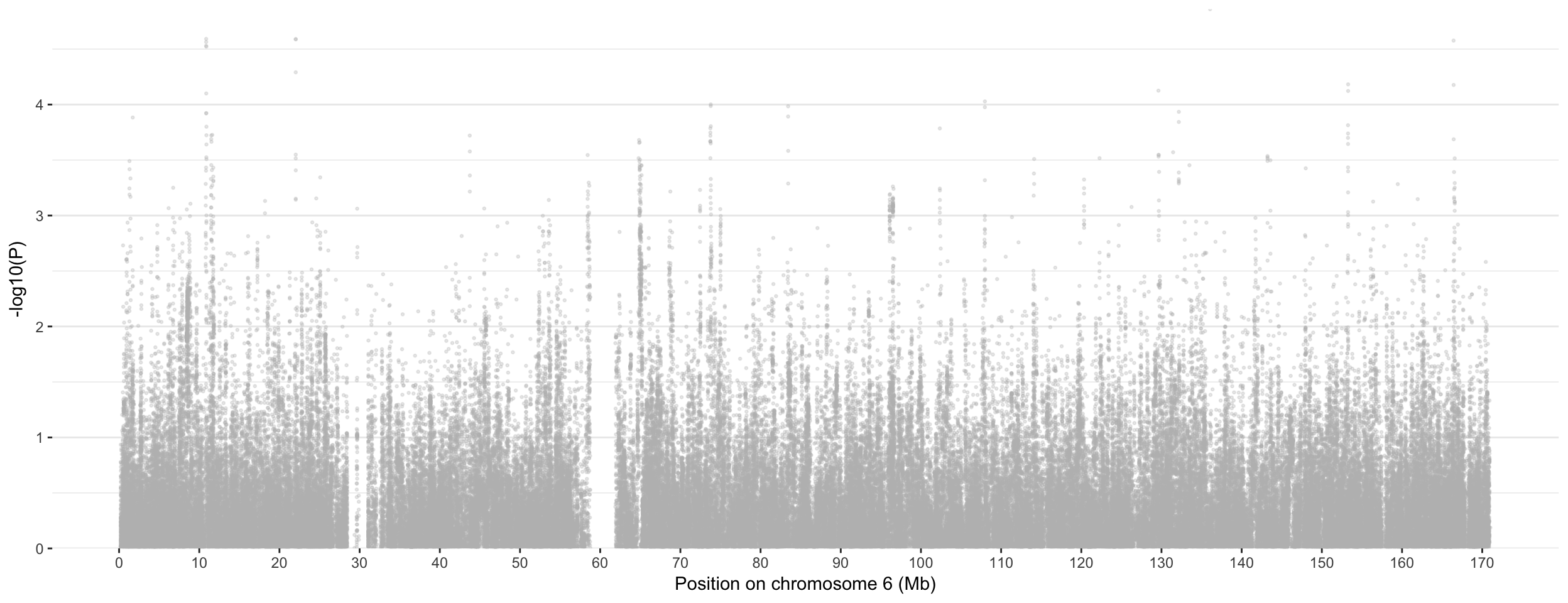
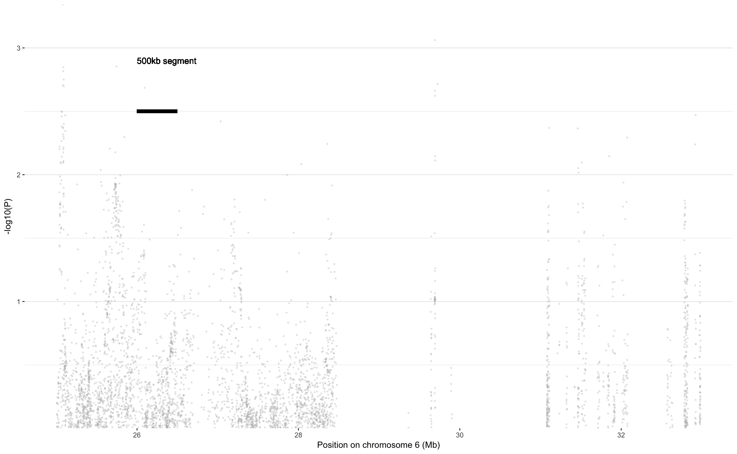
There is something weird on chromosome 6, with 70+ unique loci associated if we believe the clumping results. Let’s have a look to it:
don <- data %>%

  filter(CHR==6) %>%

  # Add clumping information
  mutate( is_major=ifelse(SNP %in% clump$SNP & P<10e-8, "yes", "no")) %>%
  mutate( is_clump=ifelse(SNP %in% Hit_SNP, "yes", "no"))

ggplot(don, aes(x=BP/1000000, y=-log10(P))) +

    # Show all points
    geom_point( aes(color=as.factor(CHR)), alpha=0.3, size=0.5, color="grey") +

    # Add highlighted points for significant association:
    geom_point(data=subset(don, is_clump=="yes"), color="orange", size=0.2) +
    geom_point(data=subset(don, is_major=="yes"), color="red", size=4) +
    geom_label_repel( data=subset(don, is_major=="yes"), aes(label=SNP), size=2) +

    # theme
    theme_bw() +
    theme(
      legend.position="none",
      panel.border = element_blank(),
      panel.grid.major.x = element_blank(),
      panel.grid.minor.x = element_blank()
    ) +
    scale_y_continuous( expand = c(0, 0) ) +
    scale_x_continuous( breaks=seq(0,200,10) ) +
    xlab("Position on chromosome 6 (Mb)")

Same thing zooming around 30 Mb. Knowing that I’ve clumped using 500kb slices! It means I should not have more than 2 distincts association in each 500kb slices. Let’s watch between 25Mb and 35Mb. This is an area of 10Mb, which is 10,000 k, which is 20 times 500kb. And I’ve way more than 20 associations here.. So what’s wrong..
don <- data %>%

  filter(CHR==6, BP>25000000, BP<33000000) %>%

  # Add clumping information
  mutate( is_major=ifelse(SNP %in% clump$SNP & P<10e-8, "yes", "no")) %>%
  mutate( is_clump=ifelse(SNP %in% Hit_SNP, "yes", "no"))

ggplot(don, aes(x=BP/1000000, y=-log10(P))) +

    # Show all points
    geom_point( aes(color=as.factor(CHR)), alpha=0.3, size=0.5, color="grey") +

    # Add highlighted points for significant association:
    geom_point(data=subset(don, is_clump=="yes"), color="orange", size=0.2) +
    geom_point(data=subset(don, is_major=="yes"), color="red", size=4) +
    geom_label_repel( data=subset(don, is_major=="yes"), aes(label=SNP), size=2) +

    # theme
    theme_bw() +
    theme(
      legend.position="none",
      panel.border = element_blank(),
      panel.grid.major.x = element_blank(),
      panel.grid.minor.x = element_blank()
    ) +
    scale_y_continuous( expand = c(0, 0) ) +
    scale_x_continuous( breaks=seq(20,40,2) ) +
    xlab("Position on chromosome 6 (Mb)") +

    #Add a segment of 500kb
    geom_segment(y=2.5, yend=2.5, x=26, xend=26.5, color="black", size=2) +
    geom_text( x=26, y=2.9, label="500kb segment", hjust=0)

Main statistics
nb_snp=nrow(data)
signif = data %>% filter(P<10e-8) %>% arrange(CHR, BP)
nb_signif=nrow(signif)
We had 2543566 in our data set. We found 569 significant association (with a 10^-8 threshold).
Here is a list of all the significant assoc:
datatable(signif, rownames = FALSE, options = list(pageLength = 5) )
Clumping details
Number of unique significant loci detected after clumping: 5 Number of loci per chromosome:
clump %>%
  group_by(CHR) %>%
  summarise( tot=n() ) %>%
  arrange(tot) %>%
  mutate(CHR=factor(CHR, CHR)) %>%
  ggplot( aes(x=CHR, y=tot)) +
    geom_segment(aes(x=CHR, xend=CHR, y=tot, yend=0), color="grey") +
    geom_point(size=4, color="orange") +
    coord_flip() +
    ylab("Number of significant loci") +
    xlab("Chromosome") +
    theme_bw()

Detail of the clumping results:
tmp <- clump %>% arrange(CHR, BP)
datatable(tmp, rownames = FALSE, filter="top", options = list(pageLength = 5) )
Pvalue distribution
data %>% ggplot(aes(x=P)) + geom_histogram(bins=200)

QQplot
qq(data$P)

Beta distribution
Should be a normal distribution centered on 0? If Beta=0, the SNP has no effect. If absolute(Beta) is strong, SNP has a strong effect.
data %>% ggplot(aes(x=BETA)) + geom_histogram(bins=200) +xlim(-2,2)

Summary table for paper
The goal is to build a table as table 2 in Naomi R. Wray et al. 2018. The fields I need are Chr, Region in Mb, SNP, location, P, A1/A2, Beta, s.e., Freq, Prev, Gene context
# We are going to use to tables: the clump data, and the GWAS result data:

# Take the useful info from the clump result. Note that the clump result has the number of lines I wanna have in my final output
output <- clump %>%
  select(SNP, CHR, BP, P, TOTAL) %>%
  arrange(CHR, BP)

# Take the useful info in the sumstat result
tmp <- data %>%
  select(SNP, A1, BETA)

# Join
output <- output %>%
  left_join( tmp, by="SNP" ) %>%
  head

# Change colnames
colnames(output) <- c("SNP", "Chr.", "Location (bp)", "P", "# of SNPs", "A1/A2", "Beta" )

# Output at .csv
write.table(output, file="TABLE/Associated_genomic_regions.csv", row.names=FALSE, quote=FALSE, sep=",")

# Show table
library(kableExtra)
options(knitr.table.format = "html")
output %>% kable() %>%
  kable_styling(bootstrap_options = "striped", full_width = F)
