GWAS on Vitamin-D: overview of Xia et al. publication
Yan Holtz, Zhihong Zhu, Julanne Frater, Perry Bartlett, Jian Yang, John McGrath
This document describes the vitamin D GWAS result of the Xia et al publication. It also reports the application of SMR and GSMR to this dataset, using Vitamin D as the risk factor, and testing its potential implication with ~80 diseases. Data downloaded from here
Manhattan
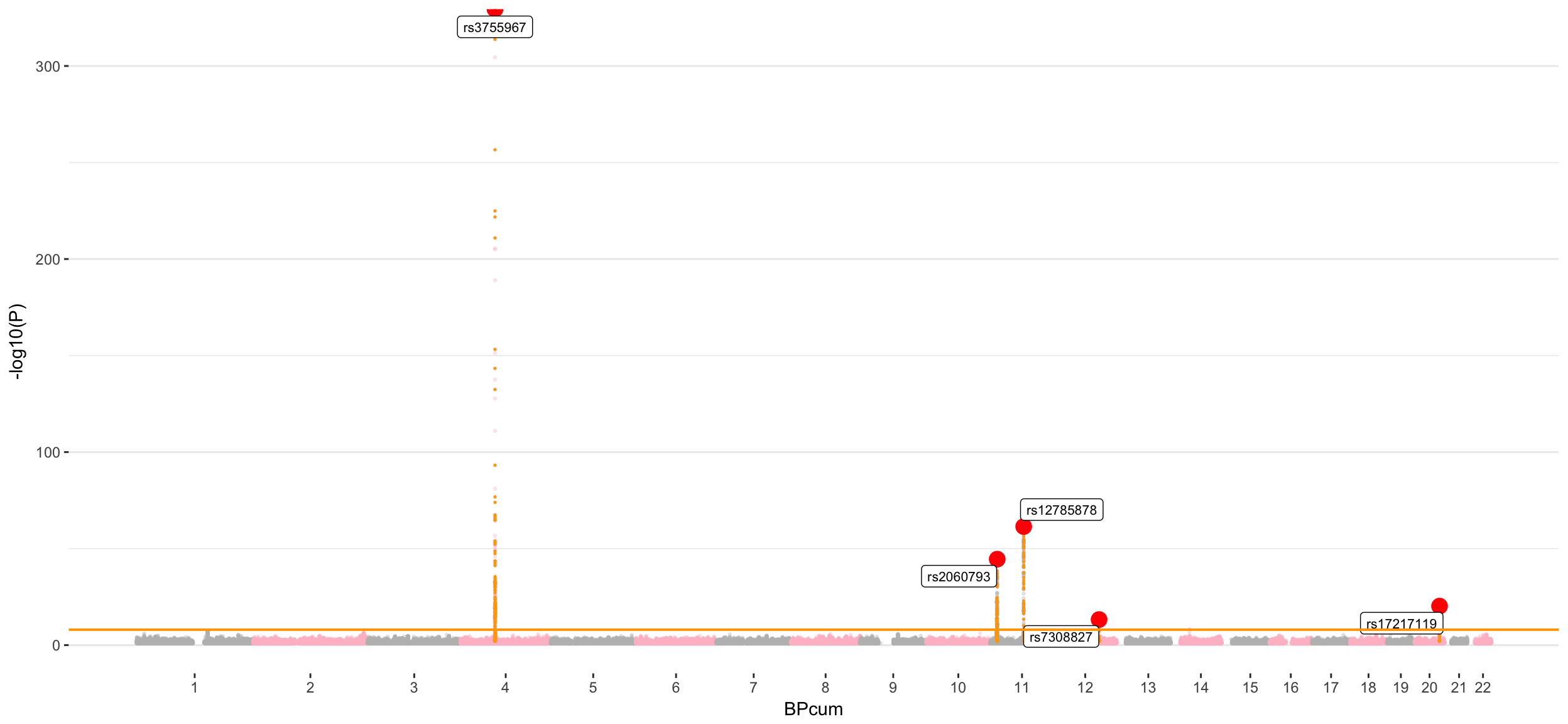
The genetic determinism of Vitamin-D appears to be oligogenic with about 6 loci involved. The association on chromosome 4 is very strong, with a -log(p-value) > 300.
# Read result
data=read_delim("0_DATA/GWAS_vitaminD_XiaEtAL.linear.gz", col_names=T, delim=" ")
data$CHR=as.factor(data$CHR)
#data=data[ sample(seq(1,nrow(data)), 10000) , ]

# Read after clumping data
clump=read.table("0_DATA/result_GWAS_VitaminD_XiaEtAl_clumped", header=T)

# A list of all SNPs implicated in an association?
Hit_SNP <- c(
  as.character(clump$SNP),
  strsplit(as.character(clump$SP2), ',', fixed=TRUE) %>% unlist() %>% gsub("\\(.\\)", "", .)
)
Hit_SNP <- Hit_SNP[Hit_SNP != "NONE"]
Classic
# -------- Add cumulative position + clumping information to data
don <- data %>%

  # Compute chromosome size and merge this info to the GWAS result
  group_by(CHR) %>%
  summarise(chr_len=max(BP)) %>%
  mutate(tot=cumsum(chr_len)-chr_len) %>%
  dplyr::select(-chr_len) %>%
  left_join(data, ., by=c("CHR"="CHR")) %>%

  # keep only SNP with pvalue < 0.05: it makes the plot realisation way faster
  filter( P<0.1 ) %>%   # | SNP %in% sample(data$SNP, 150000)

  # Add a cumulative position colummn to the data set
  arrange(CHR, BP) %>%
  mutate( BPcum=BP+tot) %>%

  # Add clumping information
  mutate( is_major=ifelse(SNP %in% clump$SNP & P<10e-8, "yes", "no")) %>%
  mutate( is_clump=ifelse(SNP %in% Hit_SNP, "yes", "no"))

# -------- prepare X axis
axisdf = don %>% group_by(CHR) %>% summarize(center=( max(BPcum) + min(BPcum) ) / 2 )

# -------- Basic plot
ggplot(don, aes(x=BPcum, y=-log10(P))) +

    # Show all points
    geom_point( aes(color=as.factor(CHR)), alpha=0.3, size=0.5) +
    scale_color_manual(values = rep(c("grey", "pink"),44)) +

    # Add highlighted points for significant association:
    geom_point(data=subset(don, is_clump=="yes"), color="orange", size=0.2) +
    geom_point(data=subset(don, is_major=="yes"), color="red", size=4) +
    geom_label_repel( data=subset(don, is_major=="yes"), aes(label=SNP), size=2.8) +

    # Make X axis:
    scale_x_continuous( label = as.character(axisdf$CHR), breaks= axisdf$center ) +

    # Signicativity line
    geom_hline(yintercept = 8, color="orange", size=0.7) +

    theme_bw() +
    theme(
      legend.position="none",
      panel.border = element_blank(),
      panel.grid.major.x = element_blank(),
      panel.grid.minor.x = element_blank()
    )
Cut X-axis and interactive
In this plot, the SNP involved in the significant associations have been removed. The idea is to focus on putative new association we will find in the UKB.
library(plotly)

don$text <- paste("SNP: ", don$SNP, "\n", "-log10(P-val): ", round(-log10(don$P),2), "\n", "Position: ", don$BP, "\n", "Chromosome: ", don$CHR, "\n", "Beta: ", don$BETA)

p <- don %>%
  filter(is_clump=="no") %>%
  filter( P<0.001 ) %>%   # | SNP %in% sample(data$SNP, 150000)

  ggplot( aes(x=BPcum, y=-log10(P), text=text)) +

    # Show all points
    geom_point( aes(color=as.factor(CHR)), alpha=0.3, size=0.5) +
    scale_color_manual(values = rep(c("grey", "pink"),44)) +

    # Make X axis:
    scale_x_continuous( label = as.character(axisdf$CHR), breaks= axisdf$center ) +

    # Signicativity line
    geom_hline(yintercept = 8, color="orange", size=0.7) +

    theme_bw() +
    theme(
      legend.position="none",
      panel.border = element_blank(),
      panel.grid.major.x = element_blank(),
      panel.grid.minor.x = element_blank()
    ) +

    ylim(0,8)

ggplotly(p, tooltip = "text")
Interactive version of the Manhattan plot. Only SNP with -log10(P) >2 & <8 are represented. Hover a point to have information concerning the SNP. Select a specific zone with your mouse to zoom on it. Be patient, there is about 40k points represented..
Detail of loci
There are 6 main associations:
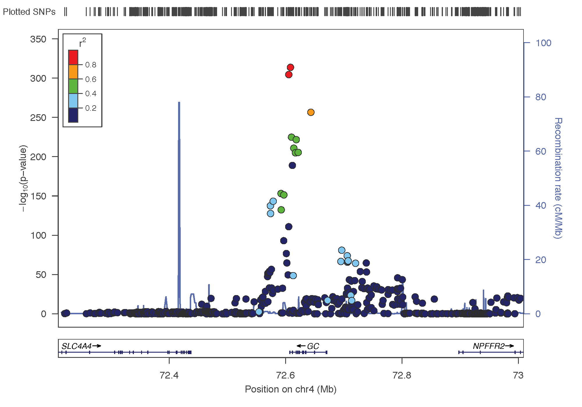
- rs3755967: chromosome 4 ~ 73Mb | gene: GC | Genome Browser | Role = Vitamin D transport.
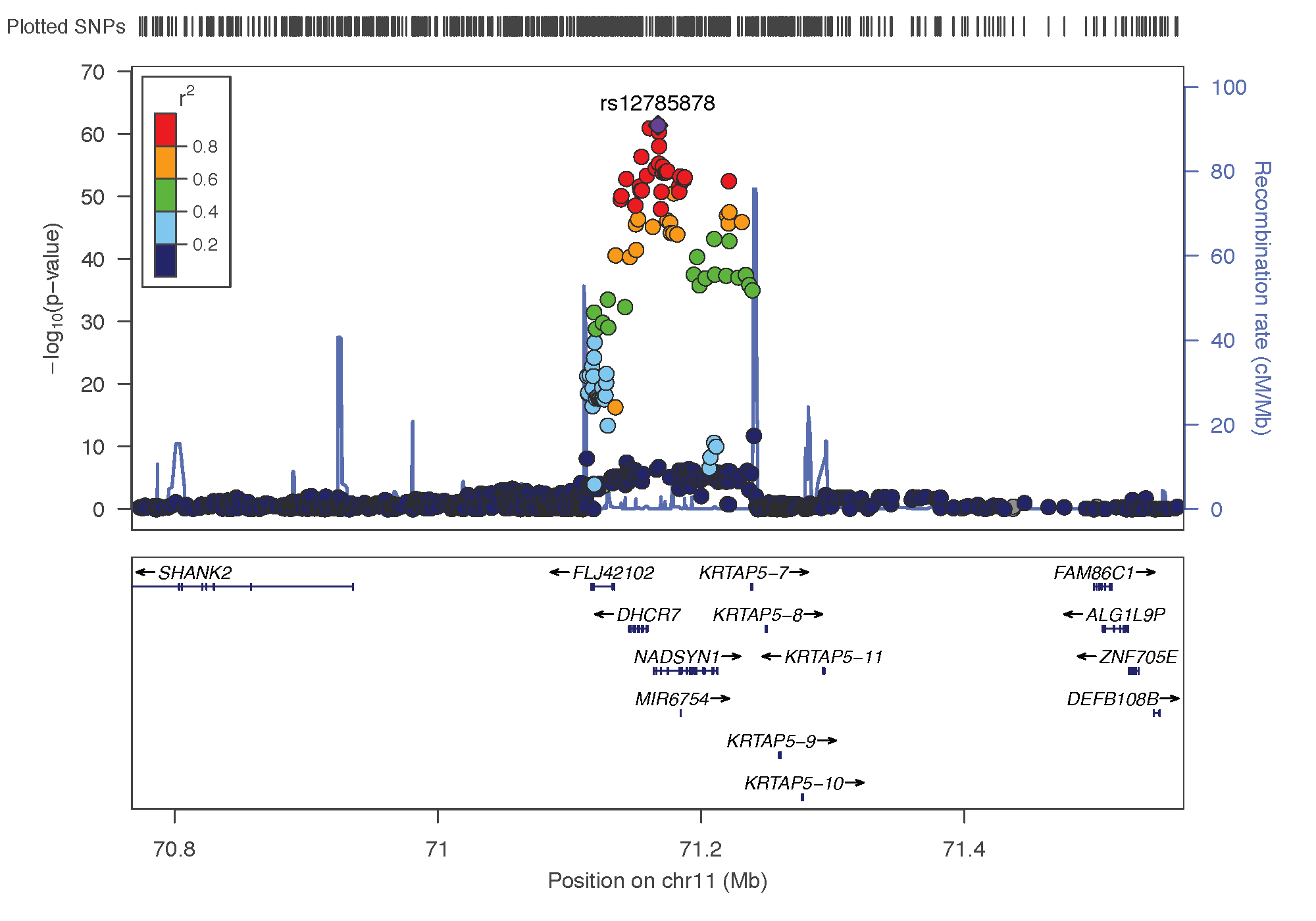
- rs12785878: chromosome 11 ~ 79Mb | gene: NADSYN1 / DHCR7 | Genome Browser
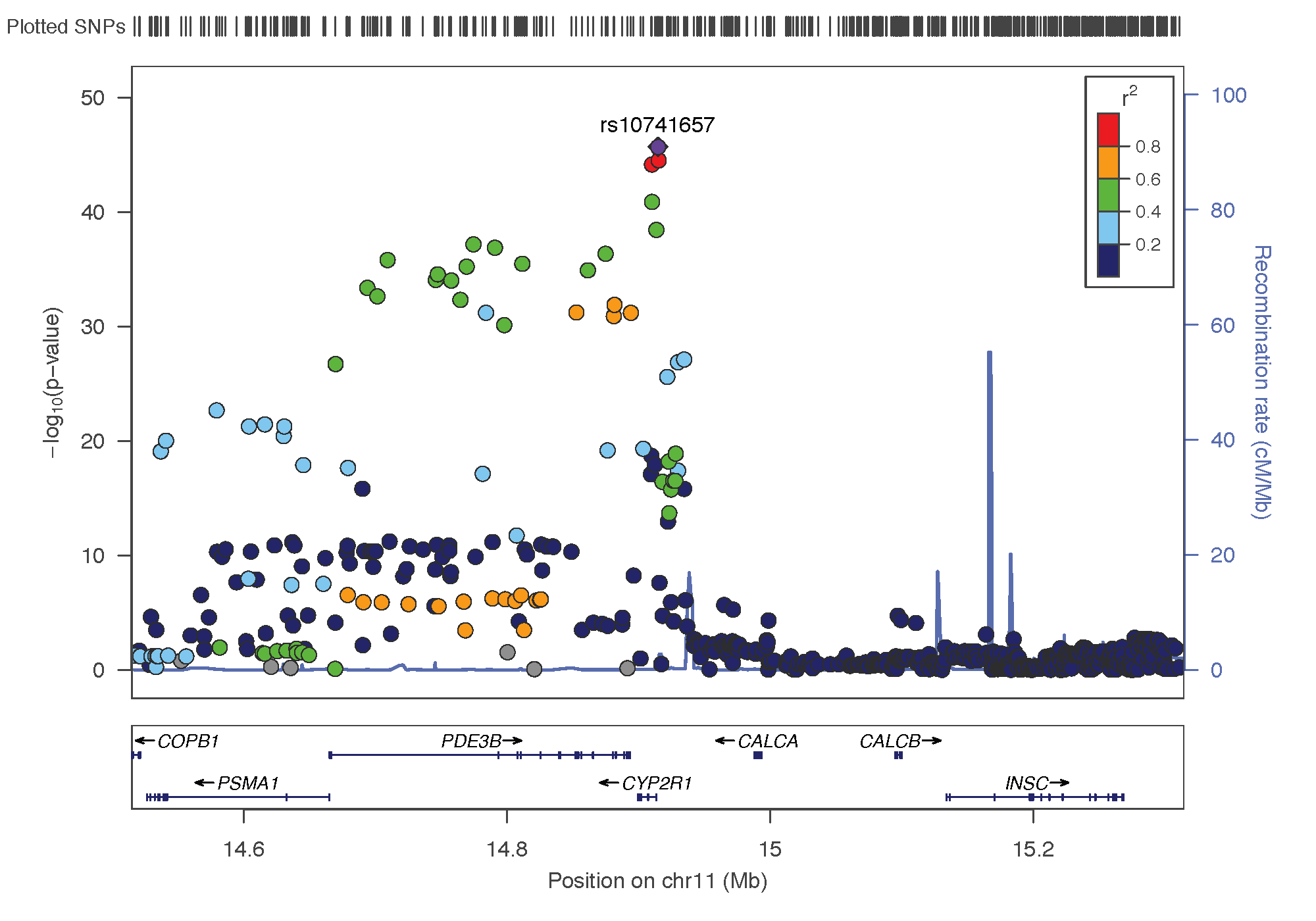
- rs10741657: chromosome 11 ~ 15Mb | gene: CYP2R1| Genome Browser | known role = hydroxylation.
- rs17216707: chromosome 20 ~ 52Mb | gene: CYP24A1| Genome Browser | Role = Catabolism.
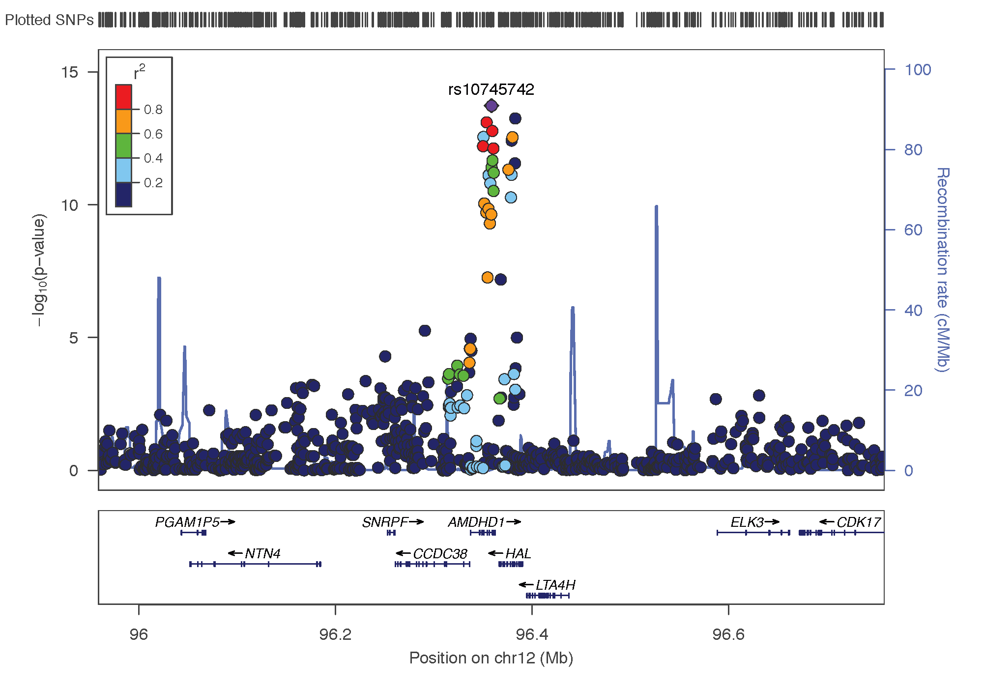
- rs10745742: chromosome 12 ~ 94Mb | gene: AMDHD1| Genome Browser
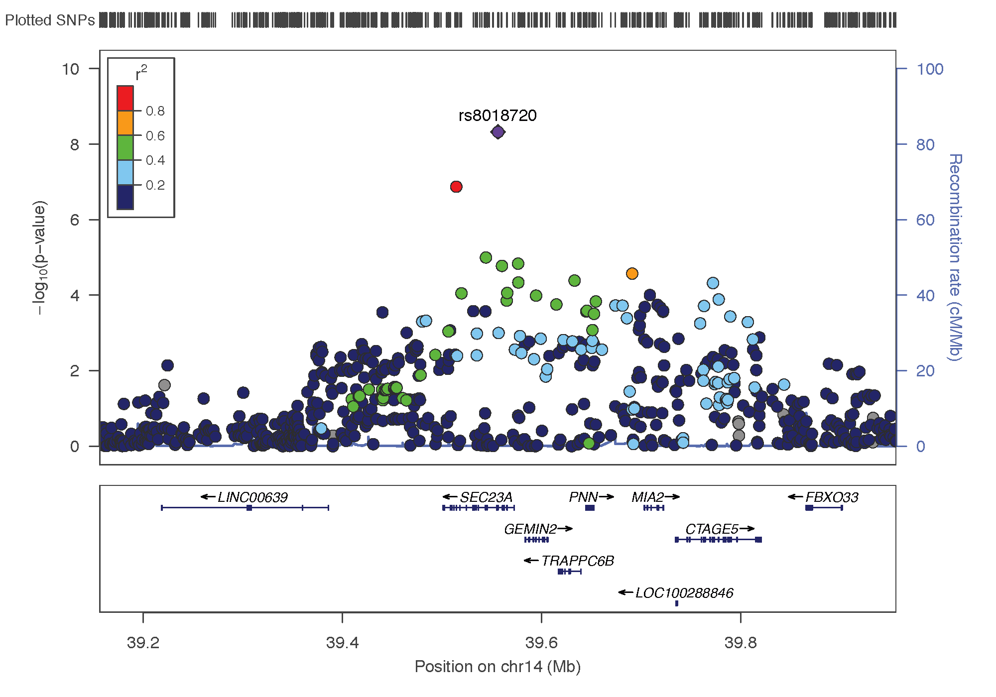
- rs8018720: chromosome 14 ~ 38Mb | gene: SEC23A| Genome Browser
Locus Zoom allows to visualise the regions of interest and see the underlying genes. Just requires the .linear result of PLINK on it, and specify the SNP of interest. Here is the result SNP per SNP:
rs3755967
rs12785878
rs10741657
rs17216707

rs10745742
rs8018720
Clumping
I run the plink clumping algorithm on this GWAS summary statistics to have an insight of the unique association loci. Here are the clumping options I’ve used. Note: GWAS summary file must NOT be zipped.
- p1 is the Significance threshold for an association
- p2 is Secondary significance threshold for clumped SNPs = SNPs that are part of the association, but not pic.
- r2 is the LD threshold for clumping and
- clump-kb is the physical distance threshold for clumping
# good folder
cd /home/y.holtz/VITAMIND_XIA_ET_AL/2_CLUMPING

# Sum stat of each chromosome
for i in $(seq 1 22) ; do
  cat /home/y.holtz/VITAMIND_XIA_ET_AL/1_GWAS/GWAS_vitaminD_XiaEtAL.linear | head -1  > file_chr_${i}
  cat /home/y.holtz/VITAMIND_XIA_ET_AL/1_GWAS/GWAS_vitaminD_XiaEtAL.linear | grep "^${i} " >> file_chr_${i}
done

# Prepare command
tmp_command="plink \
          --bfile /gpfs/gpfs01/polaris/Q0286/UKBiobank/v2EURu_HM3/ukbEURu_imp_chr{TASK_ID}_v2_HM3_QC\
          --clump file_chr_{TASK_ID} \
          --clump-p1 0.00000001 --clump-p2 0.01 --clump-r2 0 --clump-kb 1000 \
          --out /home/y.holtz/VITAMIND_XIA_ET_AL/2_CLUMPING/GWAS_vitaminD_XiaEtAL_.clump_chr{TASK_ID}"

# Send qsub
qsubshcom "$tmp_command" 1 50G clumping_plink 30:00:00 "-array=1-22"
It is more handy to have only one file with all the chromosome. Let’s build it:
# good folder
cd ~/VITAMIND_XIA_ET_AL/2_CLUMPING

# concatenate
cat *clumped | grep "CHR" | head -1 > result_GWAS_VitaminD_XiaEtAl_clumped
cat GWAS*clumped | grep -v "CHR" | sed '/^$/d' | grep -v "NA"  >> result_GWAS_VitaminD_XiaEtAl_clumped

# Transfert it locally
cd /Users/y.holtz/Dropbox/QBI/4_UK_BIOBANK_GWAS_PROJECT/VitaminD-GWAS/0_DATA
scp  y.holtz@delta.imb.uq.edu.au:/home/y.holtz/VITAMIND_XIA_ET_AL/2_CLUMPING/result_GWAS_VitaminD_XiaEtAl_clumped  .
Do I have my 6 loci after clumping?
clump=read.table("0_DATA/result_GWAS_VitaminD_XiaEtAl_clumped", header=T)
clump
FUMA
FUMA is a tool for functional mapping and annotation of genetic associations ref. A FUMA analysis of this GWAS sumstat has been run. The result is accessible here.
- Id: y.holtz@uq.edu.au
- Psw: fumayanholtz
# transfer locally for FUMA?
cd /Users/y.holtz/Desktop
scp y.holtz@delta.imb.uq.edu.au:/home/y.holtz/VITAMIND_XIA_ET_AL/1_GWAS/GWAS_vitaminD_XiaEtAL.linear.gz .
A few thoughts on the FUMA analysis:
- It looks like a lot of SNP are missing in their manhattan plot version
- Only one Genomic risk loci is reported. Chromosome 4, on SNP rs113227722 at position 71316300. It’s weird it is not the best SNP of this area. It has a very low MAF: 0.04.
- The gene-based test outputs only one significant genes: MUC7 in the chromosome 4 area. This is not what I excpected, not what is described in Xia et al.
–> These results are very weird, I need to investigate further why FUMA does not work properly.
About genes position
Xia et al. locate the SNP rs3755967 on chromosome 4, position 72,828,262 on their nature paper. I’ve read their publication several times, including supplementary data, but I didn’t see any information concerning the HG version used. After my mail they revised their data and produced a new file, with position 72,609,398
In my UKB data, this SNP rs3755967 is located at position 72,609,398. As far as I know UKB uses the Hg19 version of Human genome, which is the same as Hg37 if I understood well.
The dbSNP website tells that rs3755967 position is 71,743,681. It also says it is in the GC gene. It uses the GRCh38 version if I understood well.
The NCBI platform gives information on the gene GC: - Its position is 71,741,693 to 71,805,520 in HG 3
- Conclusion
- Vitamin-D genetic determinism appears to be oligogenic like described in Xia et al publication. 6 major loci are associated on chromosome 4, 11, 12, 14 and 20. A few other significant loci could be discovered with more detection power (+sample size). But the manhattan plot suggests an oligogenic control in any case.
Note: cleaning the GWAS sumstat:
# I download the vitamin-D summary statistics from here: https://drive.google.com/drive/folders/0BzYDtCo_doHJRFRKR0ltZHZWZjQ
# Then from local download folder to delta
gzip upload_25HydroxyVitaminD_QC.METAANALYSIS1.txt
scp upload_25HydroxyVitaminD_QC.METAANALYSIS1.txt.gz  y.holtz@delta.imb.uq.edu.au:/home/y.holtz/VITAMIND_XIA_ET_AL/1_GWAS

# good to delta folder
cd /home/y.holtz/VITAMIND_XIA_ET_AL/1_GWAS

# I miss the frequence of the major allele in this file. I can use the hapmap3 frequencies previously calculated
cat /home/y.holtz/BLOOD_GWAS/1_GWAS/PLINK/all_frequency_1.frq

# --- MA FORMAT --- make the file with this new column, transform it in a format suitable for GSMR.
echo "SNP A1 A2 freq b se p n" > GWAS_vitaminD_XiaEtAL.ma
join <(zcat upload_25HydroxyVitaminD_QC.METAANALYSIS1.txt.gz | sort -k 1,1) <(awk '{print $2, $6}' /home/y.holtz/BLOOD_GWAS/1_GWAS/PLINK/all_frequency*.frq | sort -k 1,1) | awk '{ print $1,$2,$3,$15,$4,$5,$6,$14}' >>  GWAS_vitaminD_XiaEtAL.ma

# --- LINEAR FORMAT --- make a .linear format suitable for PLINK or FUMA
echo "CHR SNP BP A1 TEST NMISS BETA STAT P" > GWAS_vitaminD_XiaEtAL.linear
zcat upload_25HydroxyVitaminD_QC.METAANALYSIS1.txt.gz | grep -v 'Chr' | awk '{ print $12, $1, $13, $2, "ADD", $14, $4, $4*$5, $6}' >> GWAS_vitaminD_XiaEtAL.linear
R  # We need to remove the 10^5 format for 100000 format
data=read.table("GWAS_vitaminD_XiaEtAL.linear", header=T)
data$BP = round(data$BP, 0)
options(scipen=500)
library(dplyr)
data <- data %>% arrange(CHR, BP)
write.table(data, file="GWAS_vitaminD_XiaEtAL.linear", quote=F, row.names=FALSE )

# --- LIGHT FORMAT --- make a light version for github
cat GWAS_vitaminD_XiaEtAL.linear | head -1 >  GWAS_vitaminD_XiaEtAL.linear.light
cat GWAS_vitaminD_XiaEtAL.linear | awk '{if( $9 < 0.1){print $0}}' >>  GWAS_vitaminD_XiaEtAL.linear.light
gzip GWAS_vitaminD_XiaEtAL.linear.light

# Transfer locally?
cd ~/Dropbox/QBI/4_UK_BIOBANK_GWAS_PROJECT/VitaminD-GWAS/0_DATA
scp y.holtz@delta.imb.uq.edu.au:/home/y.holtz/VITAMIND_XIA_ET_AL/1_GWAS/GWAS_vitaminD_XiaEtAL.linear.gz .

# Note: I need to delete 2 SNPs that have a P of 0 in the R output. Because R rounds them to 0
more GWAS_vitaminD_XiaEtAL.linear | awk '{ if($9!=0){print $0}}' | gzip > GWAS_vitaminD_XiaEtAL.linear_IGV.gz
A work by Yan Holtz
Yan.holtz.data@gmail.com